摘要

针对时延未知的带噪信号，使用广义相关算法计算时延估计。为提高估计精度，采用蒙特卡洛方法估计时延值。首先模拟建立两个带噪且互不相关的接收信号，通过广义相关算法多次实验计算时延，接着利用蒙特卡洛方法对多次实验计算得出的时延求均值，从而利用均值估计出时延。仿真实验表明，当信噪比为 $6 dB$ 时，本实验采用的方法误差为 2.27%。

Abstract

A generalized cross-correlation time delay estimation algorithm is proposed to calculate the time delay between two signals with noise and unknown delay. The Monte Carlo method is used to improve the estimation accuracy. Two irrelevant signals with noise are constructed in the simulation. Then make a few times of experiments using the generalized cross-correlation algorithm to get the delay in every experiment, and use the Monte Carlo method to calculate the mean which represents the time delay. Simulation results show that the relative error is 2.27% when the signal-to-noise ratio is 6 dB.

一、引言

时延估计是信号处理领域较为重要的问题，其在雷达[1]、声纳[2]、无线电通信[3]等领域得到广泛的应用。

经典的时延估计算法有基本相关法、广义相关算法[4]、子空间估计算法[5]和自适应算法[6]等。在高信噪比和高采样率的条件下,相关算法可以得到精确的时延估计。但其需要估计信号功率谱,只能估计采样间隔整数倍时延,且需峰值检测。子空间类算法可实现多径时延估计,但该算法需要矩阵运算,计算量大且需要峰值检测。自适应估计法需在采样间隔整数倍时延估计出后利用该算法估计出小数部分,进而提高估计精度。近年来,针对不同的应用环境,很多算法被应用于时延估计。

同时,新的信号处理算法也用于时延估计中。蒙特卡洛方法是一类非常重要的数值计算方法,它以概率统计理论为指导,使用随机数或伪随机数,采用统计抽样理论近似求解问题。其主要理论基础是概率论中的大数定律[7],其主要手段是随机变量的抽样[8]。文献[9]和文献[10]利用重要性采样(IS)的方法实现了参考信号已知条件下的非多径和多径的时延估计，进而将蒙特卡洛算法的思想应用到了时延估计中。这类算法的思想是利用蒙特卡洛(MC)方法对未知参数的分布函数抽样,计算样本均值直接得到参数估计结果,具有很好的实践意义[11]。

本文使用广义相关算法，配合蒙特卡洛方法，计算两模拟接收信号的延迟估计值，并与实际延迟进行对比，分析了该方法的误差和优缺点。

二、问题描述

时延估计所要解决的基本问题为：准确、迅速地估计和测定接收器或接收阵列接收到的同源信号之间的时间延迟。由于在接收现场可能存在各种噪声和干扰，接收到的目标信号往往淹没于噪声和干扰之中。因此，对带噪信号进行时延估计要排除噪声和干扰的影响，提高接收信号的信噪比。

三、处理方法

（一）原理

1. 基本时延估计方法

相关法是最经典的时延估计方法，它通过信号的自相关函数滞后的峰值估计信号之间延迟的时间差[12]。其基本思想是利用两信号 $x_1 (t)$ 和 $x_2 (t)$ 的相关函数来估计时间延迟。假设两接收信号为：

$x_1 (t)=s(t)+n_1 (t)$

$x_2 (t)=s(t-D)+n_2 (t)$

$x_1(t)$ 和 $x_2(t)$ 是两个相互独立的接收信号， $n_1(t)$ 和 $n_2(t)$ 为加性噪声， $D$ 为时间延迟。假定噪声均为零均值，方差等于 1 的正态平稳随机过程，且噪声之间以及信号与噪声之间相互独立，则信号的相关函数为：

$R_{12} (τ)=E[x_1 (t) x_2 (t+τ)]=R_{ss} (τ-D)+R_{sn_1} (τ-D)+R_{sn_2} (τ)+R_{n_1 n_2} (τ)$

式中，假设 $s(t)$ 、 $n_1(t)$ 和 $n_2(t)$ 三者相互独立，则有：

$R_{sn_1} (\tau-D)=0$

$R_{sn_2} (τ)=0$

$R_{n_1 n_2} (τ)=0$

即源信号与噪声之间及噪声与噪声之间完全正交，由自相关函数 $R_ss$ 的性质：

$\left \vert R_{ss} (\tau-D)\right \vert < R_{ss} (0)$

可知，当 $\tau-D=0$ 时， $R_ss$ 达到最大值，即两个接收信号的相关性最大。因此选择 $R_ss (\tau-D)$ 取得最大值的 $\tau$ 值作为时延值。相关时延估计算法计算简单、直观，但由于互相关函数受信号的谱性和噪声的影响，此方法不能兼顾时延估计值的分辨率和稳定性。

（二）广义相位谱法

广义相位谱法师基于相位谱估计的时延户籍方法中最常见的一种算法。由维纳-辛钦定理可知，信号的相关函数与其功率谱是互为傅里叶变换的。因此，信号之间的相似性既可以由相关函数在时间域比较也可以由功率谱密度函数在频率域来比较。文献[13]通过计算两个信号的互功率谱估计信号时延，采用相位数据回归法对相位数据进行处理，可以使互谱时延估计的处理结果接近甚至等效于最大似然估计器。对式 $R_(x_1 x_2 ) (τ)=R_ss (τ-D)$ 两边取傅里叶变换，有：

$G_{x_1 x_2} (f)=G_{ss} (f) e^{(-j2πjd)}=G_{ss} (f)e^{(jθ(f))}$

推导可得到：

$θ(f)=\arctan{\frac{Im[G_{x_1 x_2} (f)]}{Re[G_{x_1 x_2} (f)]}}=-2πfd$

$θ(f)$ 表示功率谱 $G_{x_1 x_2} (f)$ 的相位函数，因此时间延迟估计 $d ̂$ 可以表示成： $d ̂=-\frac{θ ̂(f)}{2πf}$ ， $θ ̂(f)$ 表示相位函数 $θ(f)$ 的估计值。

2. 蒙特卡洛方法

由于加入了噪声，所以在每次实验中计算得到的延时 $d$ 与延时实际值 $D$ 之间存在误差，可采用最小二乘法来求取时间延迟估计 $d ̂$ ，但本实验采用蒙特卡洛方法，通过多次随机实验求统计平均的方法代替最小二乘法得到时延估计，在每一次实验中，延时 $d$ 表示为： $d=-\frac{max[θ(f)]}{2πf}$ ，而时间延迟估计 $d ̂$ 表示为：

$d ̂=\frac{1}{M}\sum_{m^(M-1)}^{d(m)}$

$d(m)$ 表示第 $m$ 次实验求得的延时， $M$ 表示随机实验的次数。随机实验得到的 $d(m)$ 方差越小，实验次数 $M$ 越大，最终求出的时间延迟估计 $d ̂$ 越接近延时实际值 $D$ [14]。

（二）算法步骤

模拟两个接收信号 $x_1 (t)$ 和 $x_2 (t)$ 并求得其互功率谱 $G_{x_1 x_2} (f)$ 。
通过公式 $d=-\frac{max[θ(f)]}{2πf}$ 求得当前实验的延时 $d(m)$ 。
重复实验 $M$ 次，通过公式 $d ̂=\frac{1}{M} \sum_{m^(M-1)}^{d(m)}$ 求得时间延迟估计值 $d ̂$ 。

四、分析

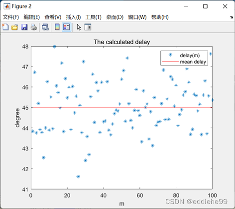
在实验中为方便可视化，使用相位延时，假设延时 $D=π⁄4$ 且接收信号为：

$x_1 (t)=sin⁡[(2πft)]+n_1 (t)$

$x_2 (t)=sin⁡[(2πft-D)]+n_2 (t)$

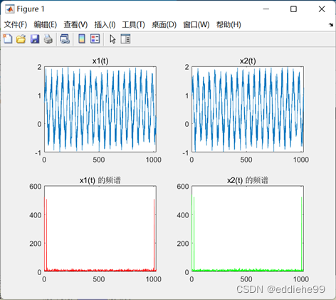
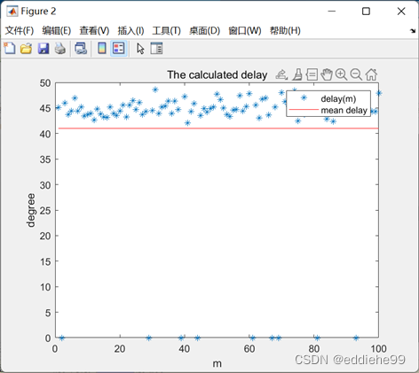
进行了 100 次随机实验，求得的延迟估计值 $d ̂=45.0130$ ，在加入了加性噪声的情况下，信噪比为 $6 dB$ ，误差为 2.27%。当信噪比降低到 $5dB$ ，误差为 8.99%，且随机实验中多次出现取 $max⁡[θ(f)]$ 计算当次实验的延时，结果等于 $0$ 的情况。当信噪比低于 $5 dB$ ，实验结果多为不可用。

五、结论

本文使用广义相关算法计算两个带噪信号的时延，并利用蒙特卡洛方法对多次实验计算得出的时延求均值，从而利用均值估计出时延。本文使用的方法优点是简单、计算复杂度低，在信噪比大于等于 $5 dB$ 的情况下，误差能控制在较低水平。缺点是没使用滤波器，依赖极值，在信噪比低的情况下结果受噪声扰动大。

六、参考文献

[1] R. Hai-Peng, L. Wen-Chao, and L. Ding, “Hopf bifurcation analysis of Chen circuit with direct time delay feedback,” Chin. Phys. B, vol. 19, no. 3, p. 030511, Mar. 2010, doi: 10.1088/1674-1056/19/3/030511.

[2] G. Carter, “Time delay estimation for passive sonar signal processing,” IEEE Trans. Acoust. Speech Signal Process., vol. 29, no. 3, pp. 463–470, Jun. 1981, doi: 10.1109/TASSP.1981.1163560.

[3] B.-W. Luo, J.-J. Dong, Y. Yu, T. Yang, and X.-L. Zhang, “Photonic multi-shape UWB pulse generation using a semiconductor optical amplifier-based nonlinear optical loop mirror,” Chin. Phys. B, vol. 22, no. 2, p. 023201, Feb. 2013, doi: 10.1088/1674-1056/22/2/023201.

[4] C. Knapp and G. Carter, “The generalized correlation method for estimation of time delay,” IEEE Trans. Acoust. Speech Signal Process., vol. 24, no. 4, pp. 320–327, Aug. 1976, doi: 10.1109/TASSP.1976.1162830.

[5] A. K. Nandi, “On the subsample time delay estimation of narrowband ultrasonic echoes,” IEEE Trans. Ultrason. Ferroelectr. Freq. Control, vol. 42, no. 6, pp. 993–1001, 1995, doi: 10.1109/58.476542.

[6] Z. Cheng and T. T. Tjhung, “A new time delay estimator based on ETDE,” IEEE Trans. Signal Process., vol. 51, no. 7, pp. 1859–1869, Jul. 2003, doi: 10.1109/TSP.2003.812735.

[7] D.-H. Duan, W. Xu, J. Su, and B.-C. Zhou, “The Stochastic stability of a Logistic model with Poisson white noise,” Chin. Phys. B, vol. 20, no. 3, p. 030501, Mar. 2011, doi: 10.1088/1674-1056/20/3/030501.

[8] X.-C. Zhang and C.-J. Guo, “Cubature Kalman filters: Derivation and extension,” Chin. Phys. B, vol. 22, no. 12, p. 128401, Dec. 2013, doi: 10.1088/1674-1056/22/12/128401.

[9] A. Masmoudi, F. Bellili, S. Affes, and A. Stephenne, “A Non-Data-Aided Maximum Likelihood Time Delay Estimator Using Importance Sampling,” IEEE Trans. Signal Process., vol. 59, no. 10, pp. 4505–4515, Oct. 2011, doi: 10.1109/TSP.2011.2161293.

[10] A. Masmoudi, F. Bellili, S. Affes, and A. Stephenne, “A Maximum Likelihood Time Delay Estimator in a Multipath Environment Using Importance Sampling,” IEEE Trans. Signal Process., vol. 61, no. 1, pp. 182–193, Jan. 2013, doi: 10.1109/TSP.2012.2222402.

[11] 李晶, 赵拥军, and 李冬海, “基于马尔科夫链蒙特卡罗的时延估计算法*,” Acta Physica Sinica, no. 13 %V. pp. 130701-1-130701–7, 2014.

[12] 行鸿彦 and 唐娟, “时延估计方法的分析,” Tech. Acoust., vol. 27, no. 1, pp. 110–114, 2008.

[13] A. Piersol, “Time delay estimation using phase data,” IEEE Trans. Acoust. Speech Signal Process., vol. 29, no. 3, pp. 471–477, Jun. 1981, doi: 10.1109/TASSP.1981.1163555.

[14] 巴斌, 郑娜娥, 朱世磊, and 胡捍英, “利用蒙特卡罗的最大似然时延估计算法,” Journal of Xi’an Jiaotong University, vol. 49, no. 8. pp. 24–30, 2015.

七、附录

fs = 1024;
D = pi / 4;
f = 20;
t = 0:1 / fs:1023 / fs;
M = 100;
noise_scale = 1.375;
delay = zeros(1, M);
mean_delay = ones(1, M);
for m = 1:Ms1 = sin(2*pi*f*t);n1 = noise_scale .* rand(fs, 1)';s2 = sin(2*pi*f*t-D);n2 = noise_scale .* rand(fs, 1)';x1 = s1 + n1;x2 = s2 + n2;X1 = fft(x1, 1024);X2 = fft(x2, 1024);subplot(2, 2, 1), plot(x1);title("x1(t)");subplot(2, 2, 3), plot(abs(X1), 'r');title("The spectrum of x1(t)");subplot(2, 2, 2), plot(x2);title("x2(t)");subplot(2, 2, 4), plot(abs(X2), 'g');title("The spectrum of x2(t)");% estimates the cross power spectral density (CPSD) of two discrete-time signalscpsd_x1_x2 = cpsd(x1, x2);d = abs(atan(imag(max(cpsd_x1_x2))/real(max(cpsd_x1_x2))));d = d * 180 / pi;delay(m) = d;
end
mean_delay = mean_delay * mean(delay);
error = abs(D*(180 / pi)-mean(delay));
relative_error = error / (D * (180 / pi));
Px2 = sum(x2.^2) / size(x2, 2);
Pn2 = sum(n2.^2) / size(n2, 2);
snr = 10 * log(Px2/Pn2);
figure
plot(delay, '*');
hold on
plot(mean_delay, 'r');
title("The calculated delay");
xlabel("m");
ylabel("degree");
legend("delay(m)", "mean delay");