让我看看是哪个小傻瓜还没用过MATLAB官方gallery，常见的图直接MATHWORKS搜索一下就能找到，一些有意思的组合图，以及一些特殊属性的设置MATHWORKS官方是有专门去整理的，虽然一些很特殊的图还是没有(哈哈哈弦图小提琴图啥的官方没有的我自己大部分都写过补充过)，但是也依旧足够收获很多了！！

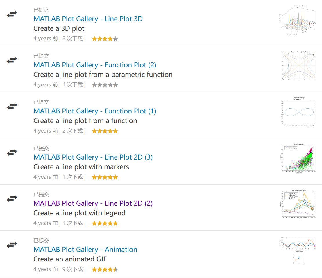
MATLAB Plot Gallery

地址：
https://ww2.mathworks.cn/products/matlab/plot-gallery.html?s_tid=srchtitle_gallery_1

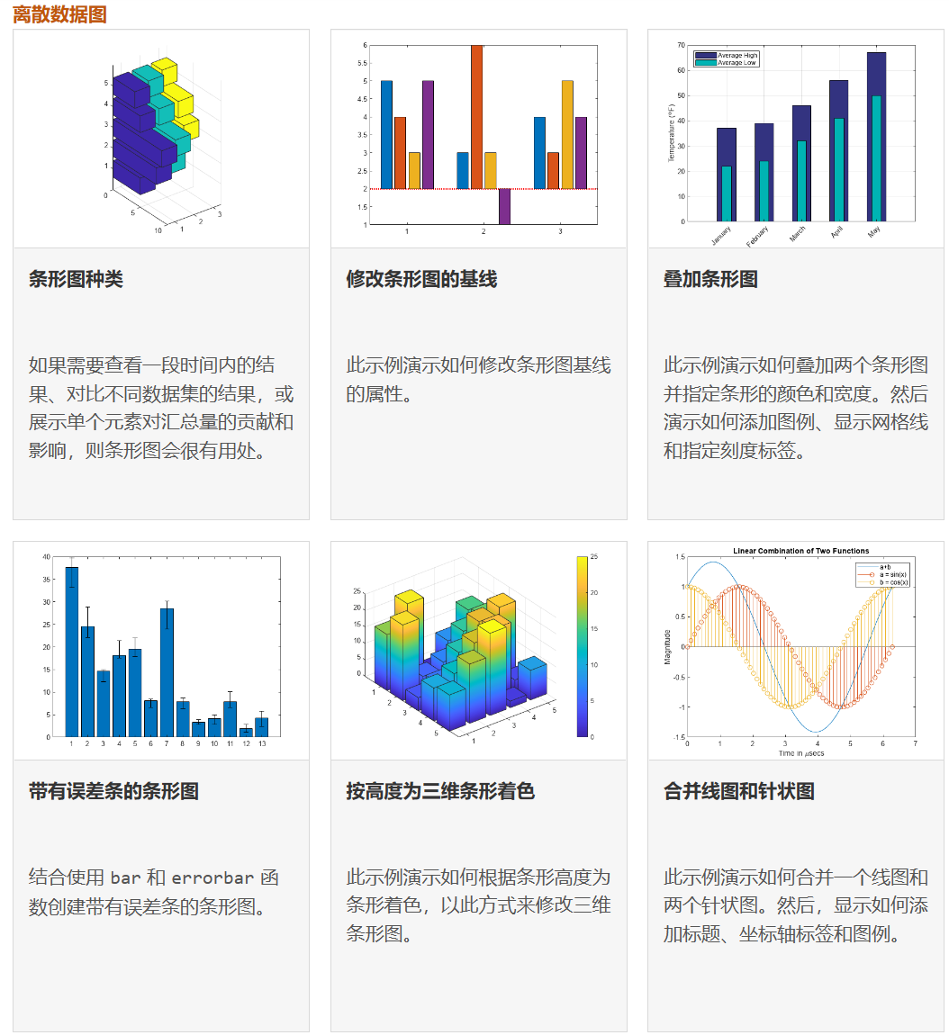
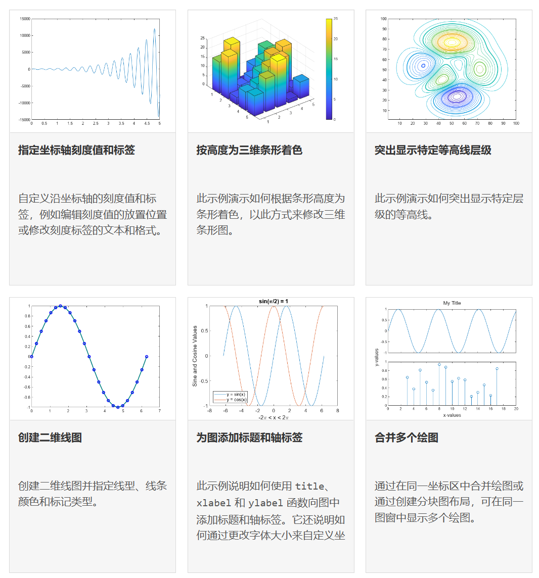
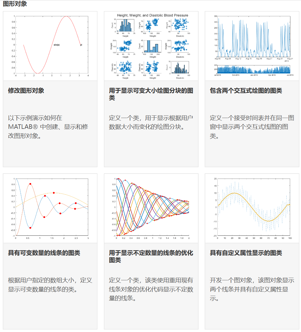
其中有超超超多优秀绘图案例：

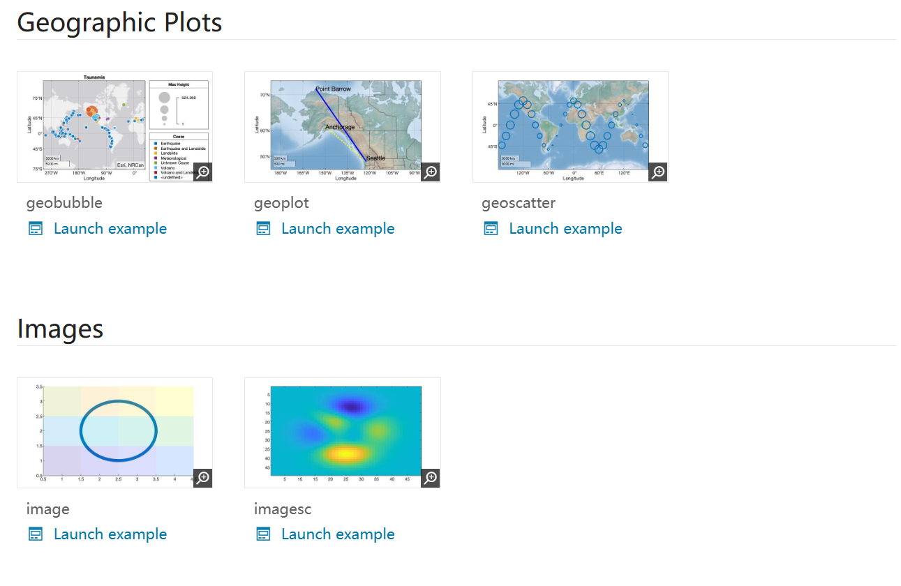
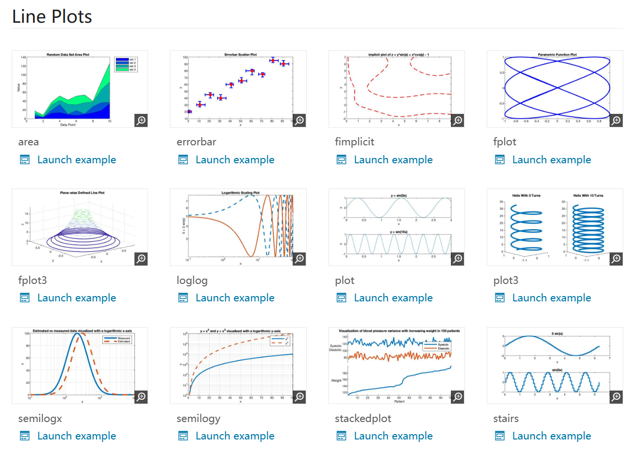
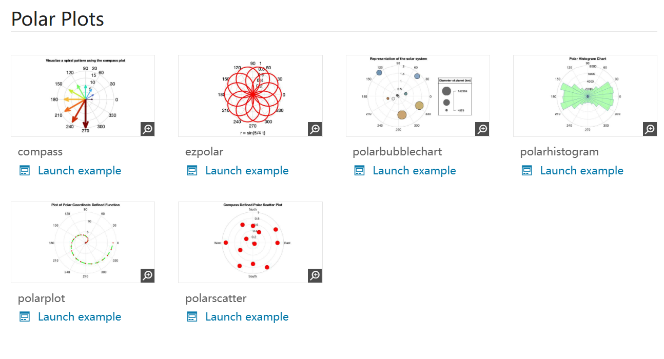
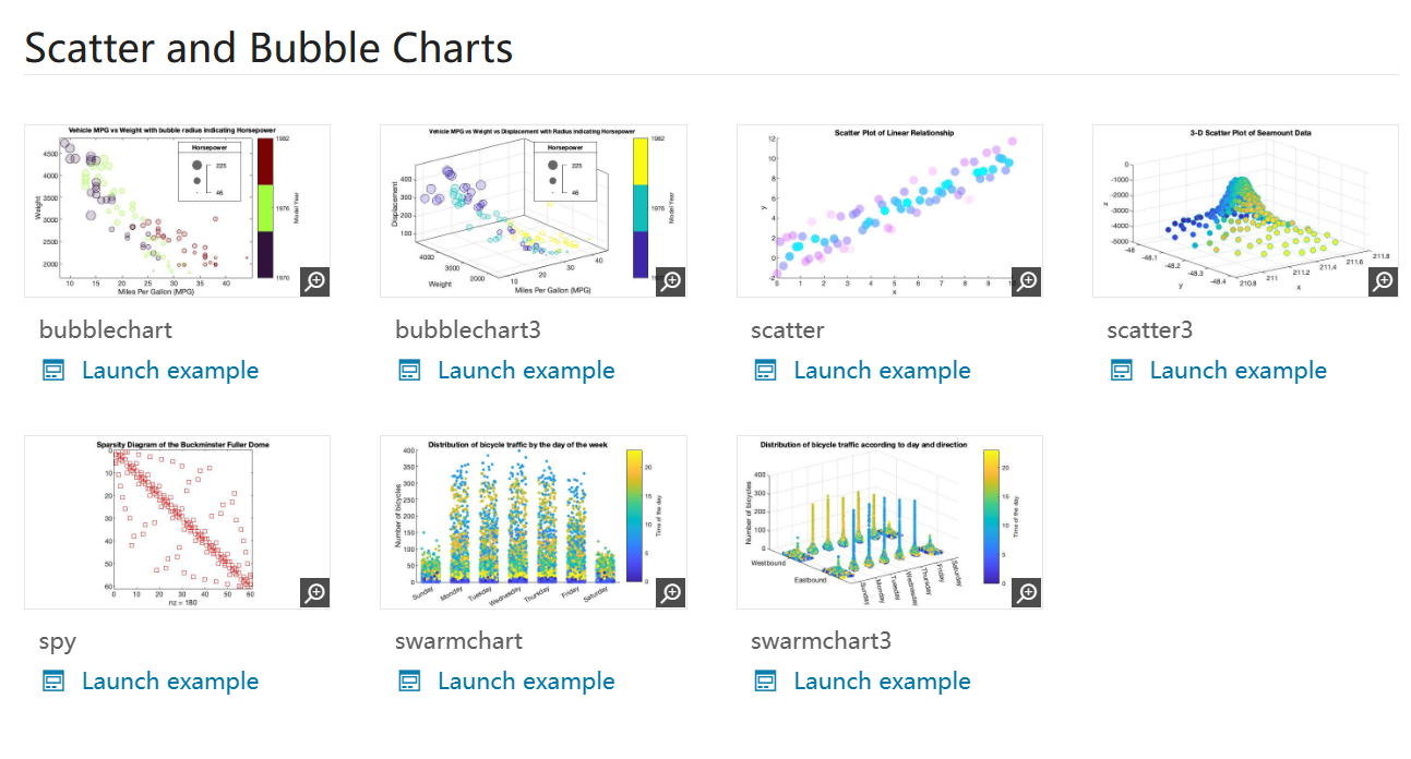
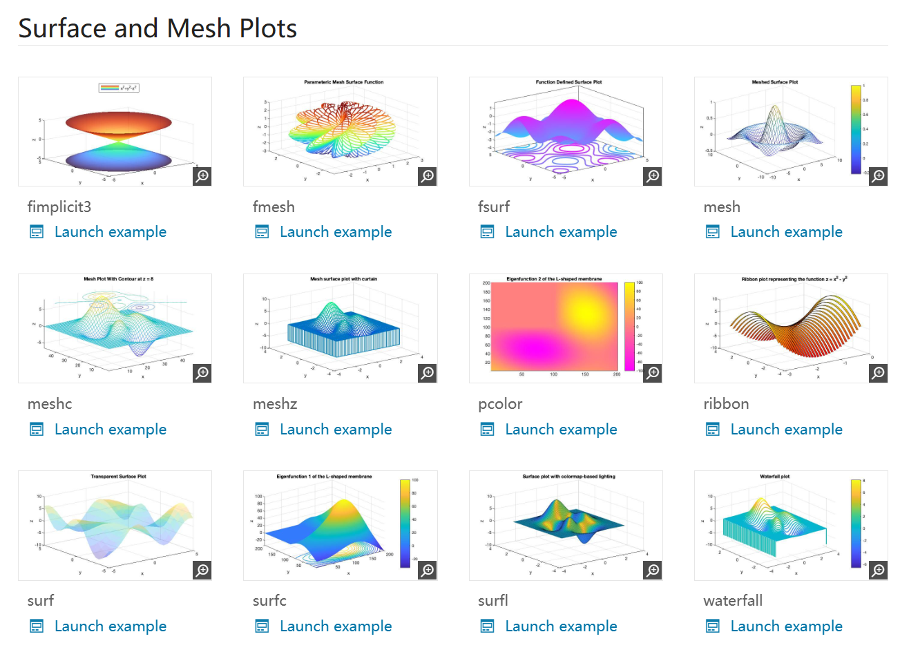
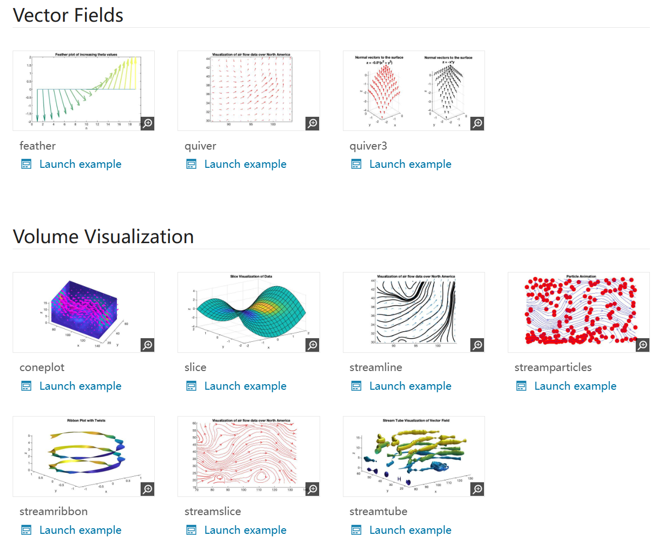
点击launch example甚至可以在线运行例子，优秀！

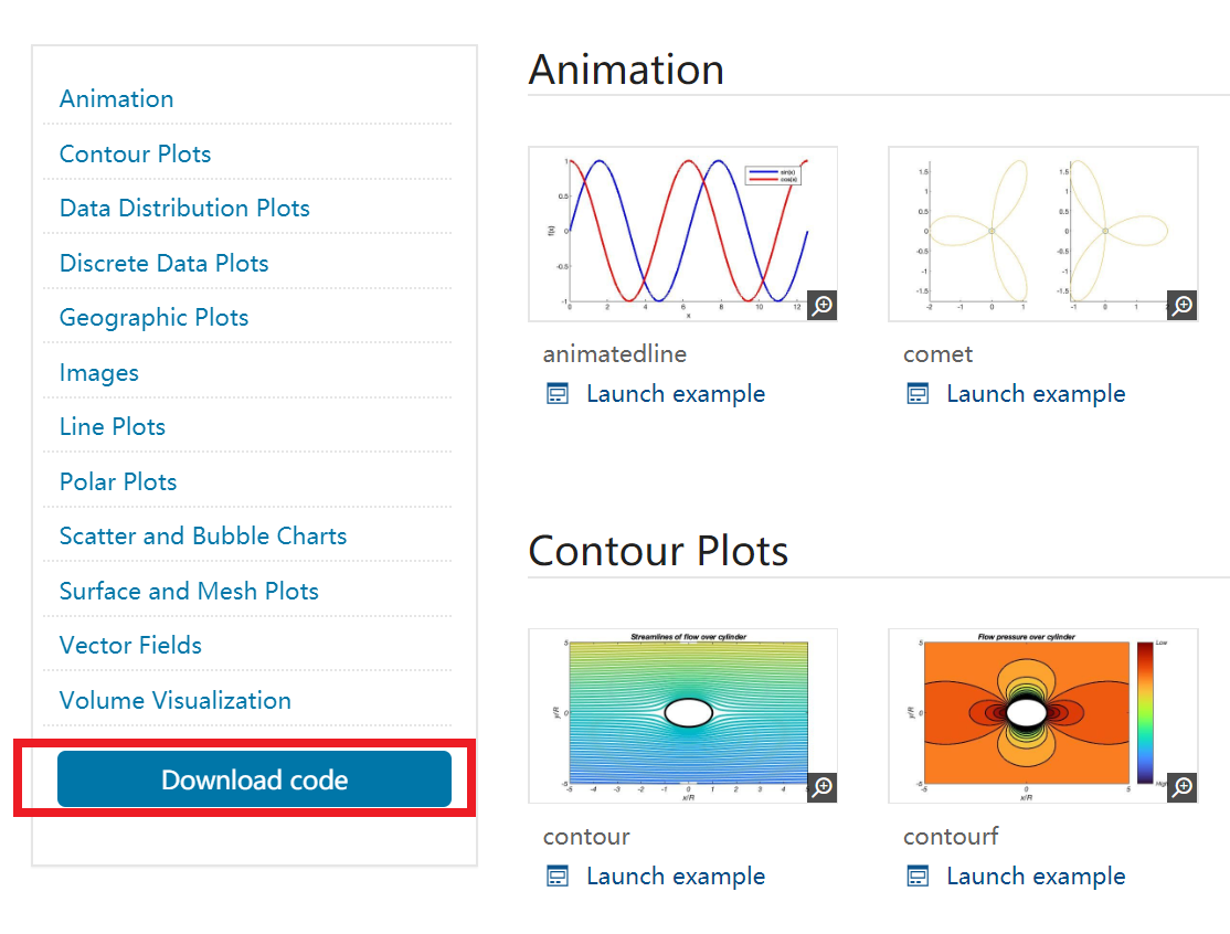
点击左侧download code可以下载全部代码及数据：

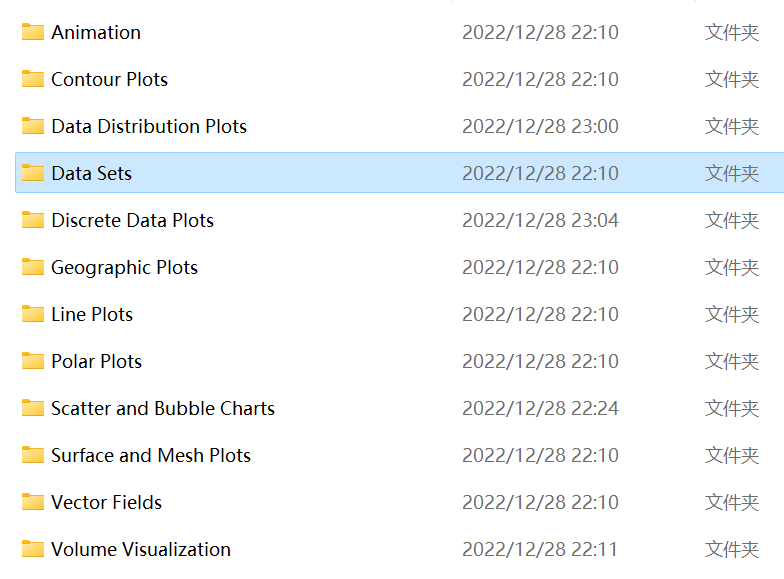
有的程序运行时会提示你没有数据，你下载的文件包内就有一个名为Data Sets的文件夹。把文件夹里的mat文件复制过去即可：

这里随便两个例子运行：

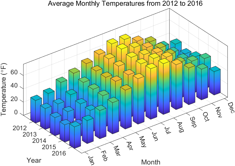
load BostonTemp.mat
yearIdx = 13;      % Choose the starting year to visualize the monthly temperature for five years.
TempData5Years = Temperatures(yearIdx:yearIdx+4,:);
barWidth = 0.5;
figure
b = bar3(TempData5Years,barWidth);      % Specify bar width in the third argumentfor k = 1:length(b)zdata = b(k).ZData;                 % Use ZData property to create color gradientb(k).CData = zdata;                 % Set CData property to Zdatab(k).FaceColor = "interp";          % Set the FaceColor to 'interp' to enable the gradient 
end
title(sprintf("Average Monthly Temperatures from %d to %d",Year(yearIdx),Year(yearIdx+4)))
xlabel("Month")
ylabel("Year")
zlabel("Temperature (\circF)")xticklabels(Months)
yticklabels(Year(yearIdx):Year(yearIdx+4))box on

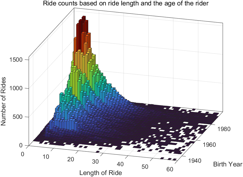
load("rideData.mat")faceColorType = "flat";
h2 = histogram2(rideData.Duration, rideData.birth_date,..."FaceColor",faceColorType);                                          % Specify the bar color schemetitle("Ride counts based on ride length and the age of the rider")
xlabel("Length of Ride")
ylabel("Birth Year")
zlabel("Number of Rides")
view(17,30)colormap("turbo"); % Specify colormap

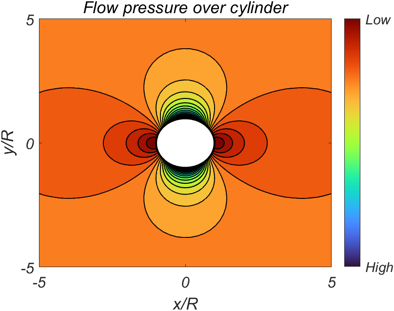
[r,theta,x,y,streamline,pressure] = flowAroundCylinder();contourLevels = 20; 
LineWidth = 1; [~,c] = contourf(x,y,pressure,...contourLevels,...              % Specify a scalar integer number of contour levels"LineWidth",LineWidth);        % Specify the contour line widthaxis([-5, 5,...     % x-axis limits -5, 5]);      % y-axis limits 
circle(0,0,1);      % Call helper function to plot circlexlabel("x/R")
ylabel("y/R")
title("Flow pressure over cylinder")set(gca,..."FontSize",15,...           % Set font size"FontAngle","italic");      % Italicize fontcolormap("turbo");    % Specify a colormap to use in the contourf plot
cb = colorbar;                  
cb.Ticks = cb.Limits;                    
cb.TickLabels = ["High" "Low"];  % Specify labels for colorbarfunction [r,theta,x,y,streamline,pressure] = flowAroundCylinder()
V_i = 1000;
a = 1;
theta = linspace(0,2*pi,100); 
rr = linspace(a,10*a,100);        
[t,r] = meshgrid(theta,rr);                        % create meshgrid in two dimensions
[x,y] = pol2cart(t,r);                             % converts polar to cartesian coordinates
streamline = V_i.*sin(t).*r.*(1-(a^2./(r.^2)));      % Creation of the streamline function
pressure = 2*(a.^2./r.^2).*cos(2.*t)-(a.^4./r.^4); % static pressure around the cylinder
endfunction h = circle(x,y,r)
hold on
th = 0:pi/50:2*pi;
xunit = r * cos(th) + x;
yunit = r * sin(th) + y;
h = plot(xunit, yunit,"-k","LineWidth",2);
hold off
end

MathWorks Plot Gallery Team

上面那些学完了没学够怎么办？？MATHWORKS官方团队MathWorks Plot Gallery Team还在fileexchange上上传了大量例子：

地址：
https://ww2.mathworks.cn/matlabcentral/profile/authors/3166380

依旧有非常多优秀例子：

随便点开一个再点击右侧下载即可：

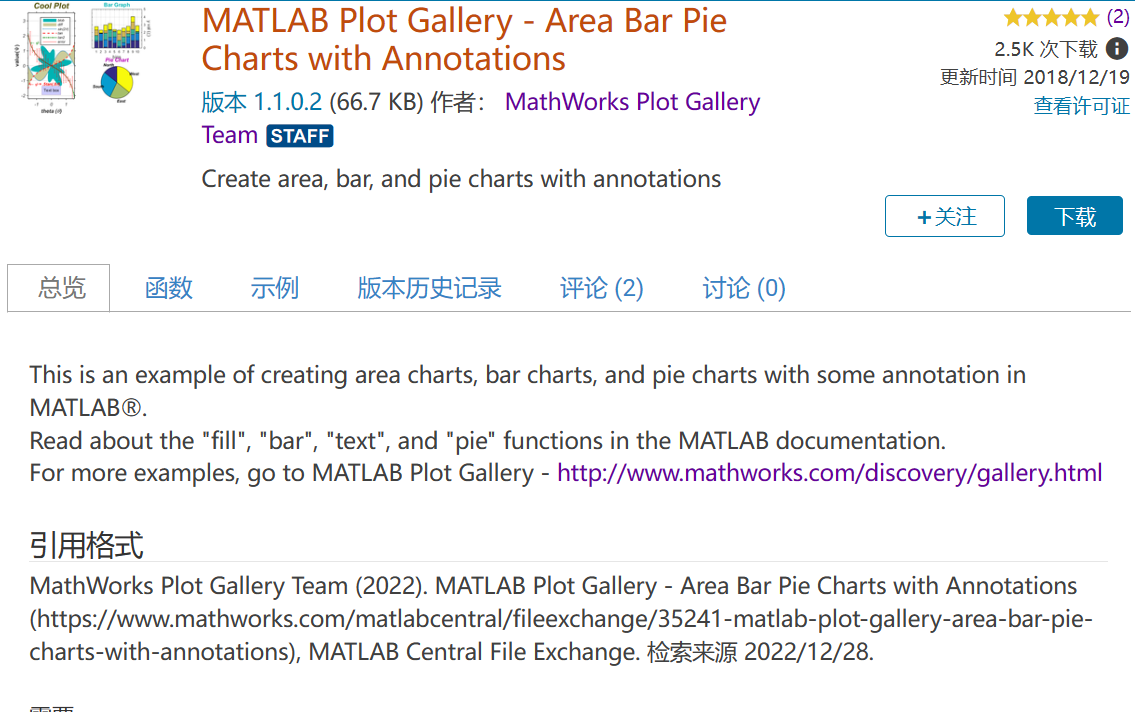
下载完直接就可以运行,以下依旧举几个例子：

%%
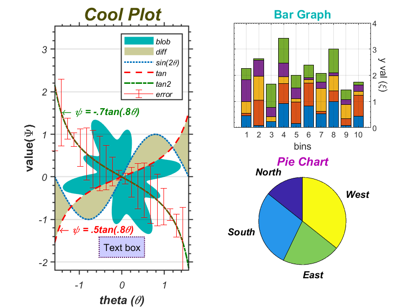
% *This is an example of creating area charts, bar charts, and pie charts with some annotation in MATLAB®* .
% 
% You can open this example in the <https://www.mathworks.com/products/matlab/live-editor.html 
% Live Editor> with MATLAB version 2016a or higher.
%
% Read about the <http://www.mathworks.com/help/matlab/ref/fill.html |fill|>, <http://www.mathworks.com/help/matlab/ref/bar.html |bar|>, <http://www.mathworks.com/help/matlab/ref/text.html |text|>, and <http://www.mathworks.com/help/matlab/ref/pie.html |pie|> functions in the MATLAB documentation.
% For more examples, go to <http://www.mathworks.com/discovery/gallery.html MATLAB Plot Gallery>
%
% Copyright 2012-2018 The MathWorks, Inc.% Set up data
t  = 0:0.01:2*pi;
x1 = -pi/2:0.01:pi/2;
x2 = -pi/2:0.01:pi/2;
y1 = sin(2*x1);
y2 = 0.5*tan(0.8*x2);
y3 = -0.7*tan(0.8*x2);
rho = 1 + 0.5*sin(7*t).*cos(3*t);
x = rho.*cos(t);
y = rho.*sin(t);% Create the left plot (filled plots, errorbars, texts)
figure
subplot(121)
hold on
h(1) = fill(x, y, [0 .7 .7]);
set(h(1), 'EdgeColor', 'none')h(2) = fill([x1, x2(end:-1:1)], [y1, y2(end:-1:1)], [.8 .8 .6]);
set(h(2), 'EdgeColor', 'none')h(3) = line(x1, y1, 'LineWidth', 1.5, 'LineStyle', ':');
h(4) = line(x2, y2, 'Linewidth', 1.5, 'LineStyle', '--', 'Color', 'red');
h(5) = line(x2, y3, 'Linewidth', 1.5, 'LineStyle', '-.', 'Color', [0 .5 0]);% Create error bars
err = abs(y2-y1);
hh = errorbar(x2(1:15:end), y3(1:15:end), err(1:15:end), 'r');
h(6) = hh(1);% Create annotations
text(x2(15), y3(15), '\leftarrow \psi = -.7tan(.8\theta)', ...'FontWeight', 'bold', 'FontName', 'times-roman', ...'Color', [0 0.5 0], 'FontAngle', 'italic')
text(x2(10), y2(10),'\leftarrow \psi = .5tan(.8\theta)', ...'FontWeight', 'bold', 'FontName', 'times-roman',...'Color', 'red', 'FontAngle', 'italic')text(0, -1.65, 'Text box', 'EdgeColor', [.3 0 .3], ...'HorizontalAlignment', 'center', ...'VerticalAlignment', 'middle', 'LineStyle', ':', ...'FontName', 'palatino', 'Margin', 4, 'BackgroundColor', [.8 .8 1], ...'LineWidth', 1)% Adjust axes properties
axis equal
set(gca, 'Box', 'on', 'LineWidth', 1, 'Layer', 'top', ...'XMinorTick', 'on', 'YMinorTick', 'on', 'XGrid', 'off', 'YGrid', 'on', ...'TickDir', 'out', 'TickLength', [.015 .015], 'XLim', x1([1,end]),...'FontName', 'avantgarde', 'FontSize', 10, 'FontWeight', 'normal', ...'FontAngle', 'italic')xlabel('theta (\theta)', 'FontName', 'bookman', 'FontSize', 12, ...'FontWeight', 'bold')
ylabel('value(\Psi)', 'FontName', 'helvetica', 'FontSize', 12, ...'FontWeight', 'bold', 'FontAngle', 'normal')
title('Cool Plot', 'FontName','palatino', 'FontSize', 18, ...'FontWeight', 'bold', 'FontAngle', 'italic', 'Color', [.3 .3 0])
legh = legend(h, 'blob', 'diff', 'sin(2\theta)', 'tan', 'tan2', 'error');
set(legh, 'FontName', 'helvetica', 'FontSize', 8, 'FontAngle', 'italic')% Create the upper right plot (bar chart)
subplot(222)
bar(rand(10,5), 'stacked')
set(gca, 'Box', 'on', 'LineWidth', .5, 'Layer', 'top', ...'XMinorTick', 'on', 'YMinorTick', 'on', 'XGrid', 'on', 'YGrid', 'on', ...'TickDir', 'in', 'TickLength', [.015 .015], 'XLim', [0 11], ...'FontName', 'helvetica', 'FontSize', 8, 'FontWeight', 'normal', ...'YAxisLocation', 'right')
xlabel('bins', 'FontName', 'avantgarde', 'FontSize', 10, ...'FontWeight', 'normal')
yH = ylabel('y val (\xi)', 'FontName', 'bookman', 'FontSize', 10, ...'FontWeight', 'normal');
set(yH, 'Rotation', -90, 'VerticalAlignment', 'bottom')
title('Bar Graph', 'FontName', 'times-roman', 'FontSize', 12, ...'FontWeight', 'bold', 'Color', [0 .7 .7])% Create the bottom right plot (pie chart)
subplot(224)
pie([2 4 3 5], {'North', 'South', 'East', 'West'})
tP = get(get(gca, 'Title'), 'Position');
set(get(gca, 'Title'), 'Position', [tP(1), 1.2, tP(3)])
title('Pie Chart', 'FontName', 'avantgarde', 'FontSize', 12, ...'FontWeight', 'bold', 'FontAngle', 'italic', 'Color', [.7 0 .7])
th = findobj(gca, 'Type', 'text');
set(th, 'FontName', 'bookman', 'FontWeight', 'bold', 'FontAngle', 'italic')

%%
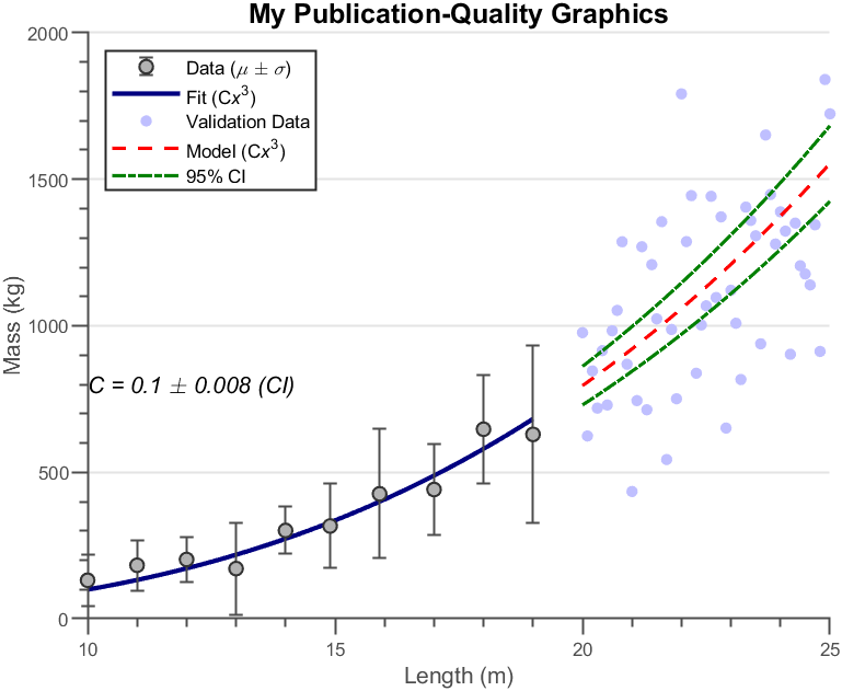
% *This is an example of how to customize a plot to make them publication quality in MATLAB®* .
%
% You can open this example in the <https://www.mathworks.com/products/matlab/live-editor.html 
% Live Editor> with MATLAB version 2016a or higher.
%
% For more examples, go to <http://www.mathworks.com/discovery/gallery.html MATLAB Plot Gallery>
%
% Copyright 2012-2018 The MathWorks, Inc.% Load data
load data xfit yfit xdata_m ydata_m ydata_s xVdata yVdata xmodel ymodel ...ymodelL ymodelU c cint% Create basic plot
figure
hold on
hFit = line(xfit  , yfit);
hE = errorbar(xdata_m, ydata_m, ydata_s);
hData = line(xVdata, yVdata);
hModel = line(xmodel, ymodel);
hCI(1) = line(xmodel, ymodelL);
hCI(2) = line(xmodel, ymodelU);% Adjust line properties (functional)
set(hFit, 'Color', [0 0 .5])
set(hE, 'LineStyle', 'none', 'Marker', '.', 'Color', [.3 .3 .3])
set(hData, 'LineStyle', 'none', 'Marker', '.')
set(hModel, 'LineStyle', '--', 'Color', 'r')
set(hCI(1), 'LineStyle', '-.', 'Color', [0 .5 0])
set(hCI(2), 'LineStyle', '-.', 'Color', [0 .5 0])% Adjust line properties (aesthetics)
set(hFit, 'LineWidth', 2)
set(hE, 'LineWidth', 1, 'Marker', 'o', 'MarkerSize', 6, ...'MarkerEdgeColor', [.2 .2 .2], 'MarkerFaceColor' , [.7 .7 .7])
set(hData, 'Marker', 'o', 'MarkerSize', 5, ...'MarkerEdgeColor', 'none', 'MarkerFaceColor', [.75 .75 1])
set(hModel, 'LineWidth', 1.5)
set(hCI(1), 'LineWidth', 1.5)
set(hCI(2), 'LineWidth', 1.5)% Add labels
hTitle = title('My Publication-Quality Graphics');
hXLabel = xlabel('Length (m)');
hYLabel = ylabel('Mass (kg)');% Add text
hText = text(10, 800, ...sprintf('{\\itC = %0.1g \\pm %0.1g (CI)}', c, cint(2)-c));% Add legend
hLegend = legend([hE, hFit, hData, hModel, hCI(1)], ...'Data ({\it\mu} \pm {\it\sigma})', 'Fit (C{\itx}^3)', ...'Validation Data', 'Model (C{\itx}^3)', '95% CI', ...'Location', 'NorthWest');% Adjust font
set(gca, 'FontName', 'Helvetica')
set([hTitle, hXLabel, hYLabel, hText], 'FontName', 'AvantGarde')
set([hLegend, gca], 'FontSize', 8)
set([hXLabel, hYLabel, hText], 'FontSize', 10)
set(hTitle, 'FontSize', 12, 'FontWeight' , 'bold')% Adjust axes properties
set(gca, 'Box', 'off', 'TickDir', 'out', 'TickLength', [.02 .02], ...'XMinorTick', 'on', 'YMinorTick', 'on', 'YGrid', 'on', ...'XColor', [.3 .3 .3], 'YColor', [.3 .3 .3], 'YTick', 0:500:2500, ...'LineWidth', 1)

%%
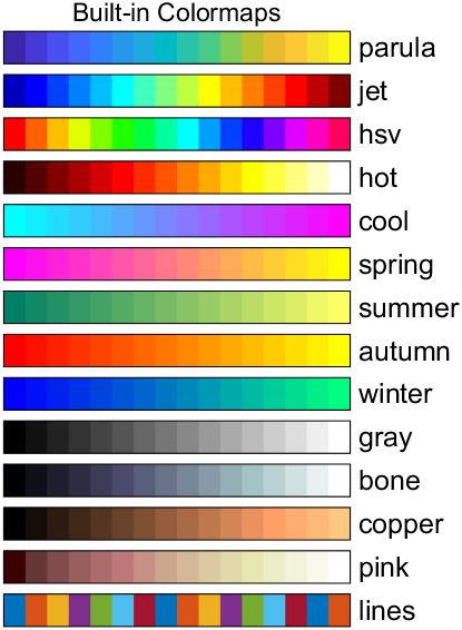
% *This is an example of creating a chart of built-in colormaps in MATLAB®* .
% 
% You can open this example in the <https://www.mathworks.com/products/matlab/live-editor.html 
% Live Editor> with MATLAB version 2016a or higher.
%
% Read about the <http://www.mathworks.com/help/matlab/ref/colormap.html |colormap|> function in the MATLAB documentation.
% For more examples, go to <http://www.mathworks.com/discovery/gallery.html MATLAB Plot Gallery>
%
% Copyright 2012-2018 The MathWorks, Inc.% Define built-in colormaps
maps = {};
if exist('parula', 'file')maps = {'parula'};
end
maps = [maps 'jet', 'hsv', 'hot', 'cool', 'spring', 'summer', 'autumn', ...'winter', 'gray', 'bone', 'copper', 'pink', 'lines'];% Number of color levels to create
nLevels = 16;figure% X data points for color patches
xData = [linspace(0, 15, nLevels); linspace(1, 16, nLevels); ...linspace(1, 16, nLevels); linspace(0, 15, nLevels)];% Create each color bar
for iMap = 1:length(maps)offset = 2*(length(maps) - iMap);yData = [zeros(2, nLevels); 1.5*ones(2, nLevels)] + offset;% Construct appropriate colormap.cData = feval(maps{iMap}, nLevels);% Display colormap chartpatch('XData', xData, 'YData', yData, ...'EdgeColor', 'none', ...'FaceColor', 'flat', ...'FaceVertexCData', cData)rectangle('Position', [0, offset, 16, 1.5], ...'Curvature', [0 0])text(16, offset, sprintf(' %s', maps{iMap}), ...'VerticalAlignment', 'bottom', ...'FontSize', 12)
endaxis equal off
title('Built-in Colormaps')

图形示例

如果是刚入门的选手，觉得上面那些都太难怎么办？？基础入门图形示例模块来啦~

地址：
https://ww2.mathworks.cn/help/matlab/examples.html?category=graphics&exampleproduct=all&s_tid=CRUX_lftnav

更多的基础教程！！

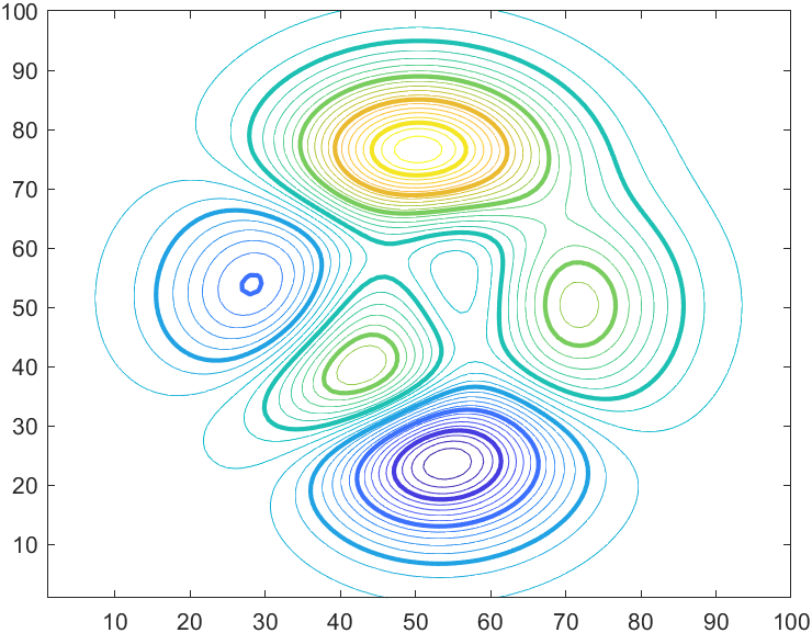
继续随便运行点示例，美滋滋：

Z = peaks(100);
zmin = floor(min(Z(:))); 
zmax = ceil(max(Z(:)));
zinc = (zmax - zmin) / 40;
zlevs = zmin:zinc:zmax;figure
contour(Z,zlevs)zindex = zmin:2:zmax;hold on
contour(Z,zindex,'LineWidth',2)
hold off

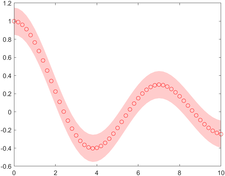
x = 0:0.2:10;                     
y = besselj(0, x);xconf = [x x(end:-1:1)] ;         
yconf = [y+0.15 y(end:-1:1)-0.15];figure
p = fill(xconf,yconf,'red');
p.FaceColor = [1 0.8 0.8];      
p.EdgeColor = 'none';           hold on
plot(x,y,'ro')
hold off

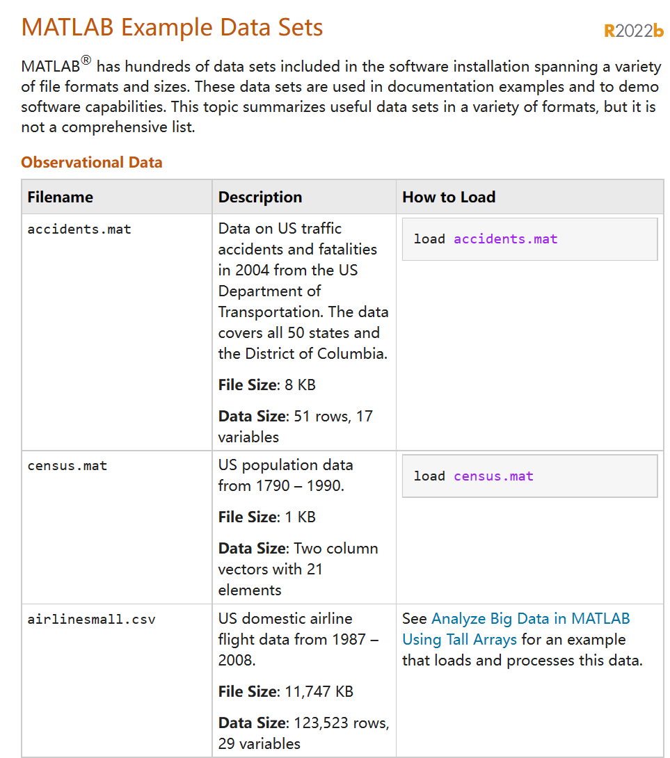
MATLAB样本数据集

想找点示例数据练练手？？来瞅瞅MATLAB都有那些自带数据集吧！

地址：
https://ww2.mathworks.cn/help/matlab/import_export/matlab-example-data-sets.html

包含了MATLAB内置数据集及其介绍：

当然也可以通过命令行窗口运行以下代码进入demos文件夹：

winopen(fullfile(matlabroot,'toolbox','matlab','demos'))

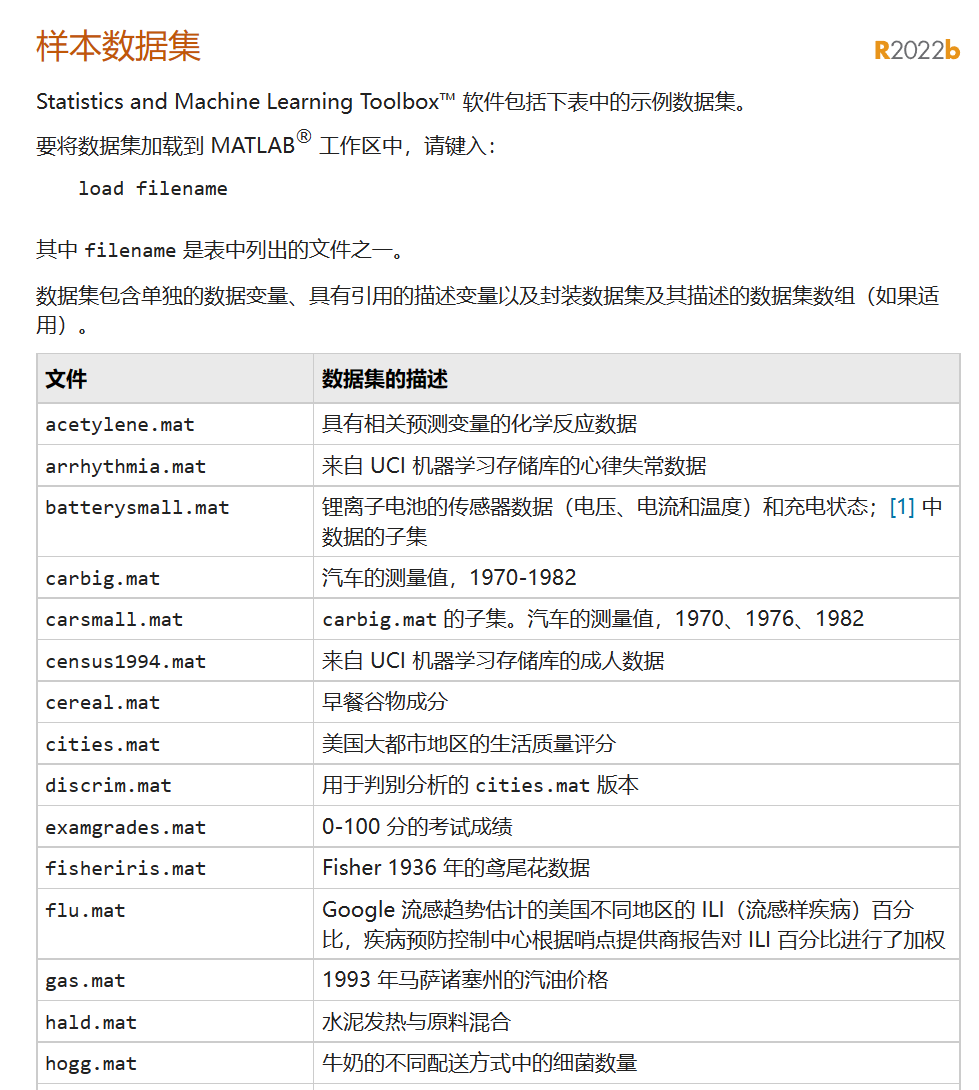
如果下载过Statistics and Machine Learning Toolbox工具箱，那么会额外拥有一些这个工具箱内置的数据：

地址：
https://ww2.mathworks.cn/help/stats/sample-data-sets.html

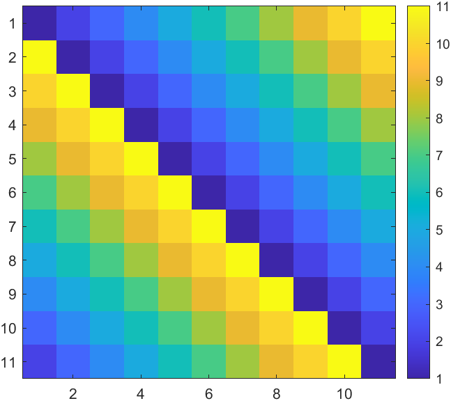
测试矩阵gallery

想要画好图怎么能不熟练掌握各种特殊矩阵？
没错MATLAB还有官方测试矩阵gallery

地址：
https://ww2.mathworks.cn/help/matlab/ref/gallery.html?searchHighlight=gallery&s_tid=srchtitle_gallery_1

比如说创建一个11阶循环矩阵：

C=gallery('circul',11);imagesc(C)
axis square
colorbar

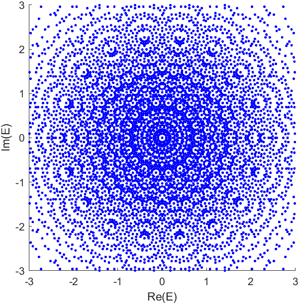
通过循环矩阵计算复平面上的特征值分布：

E = zeros(18,20000);rng('default')
for i = 1:20000x = -0.4 + 0.8*randi([0 1],1,18);A = gallery('circul',x);E(:,i) = eig(A);
endscatter(real(E(:)),imag(E(:)),'b.')
xlabel('Re(E)')
ylabel('Im(E)')
xlim([-3 3])
ylim([-3 3])
axis square

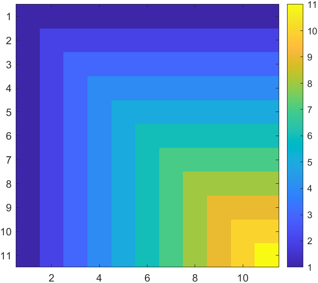
11阶minij矩阵：

M=gallery('minij',11);imagesc(M)
axis square
colorbar

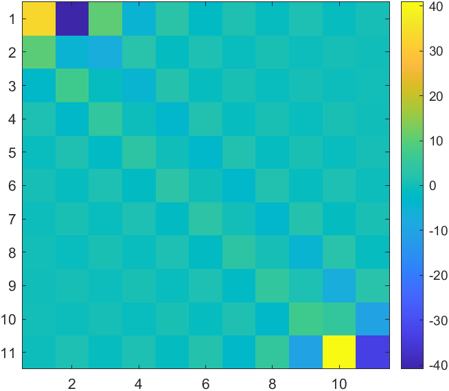
Chebyshev 谱微分矩阵:

C=gallery('chebspec',11,0);imagesc(C)
axis square
colorbar

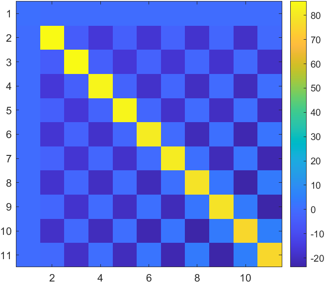
矩阵条件数估计量的反例:

C=gallery('condex',11);imagesc(C)
axis square
colorbar

完

上面这些都学完我就不信还有人不会绘图hiahiahia