本文选自论文：Range Doppler Detection for automotive FMCW Radars
论文作者：Volker Winkler
DICE GmbH & Co KG Majority owned by Infineon Technologies Freistaedterstrasse 400, 4040 Linz, Austria
本文由 @Leela梨辣 提供，由 @调皮连续波 翻译整理，仅供雷达专业人士及爱好者研究学习。
本文编辑：调皮哥的小助理

摘要

The FMCW-Radar-Principle is widely used for automotive radar systems. The basic idea for FMCW-Radars is to generate a linear frequency ramp as transmit signal. The difference frequency between the transmitted and received signal is determined after downconversion. In order to detect range and velocity together, the information, extracted from one frequency ramp, is not enough, becaus it is ambiguous. Several subsequent ramps have to be generated to remove the ambiguity between the frequency portion produced by range and the doppler frequency.

译文：FMCW雷达原理广泛应用于汽车雷达系统，FMCW雷达的基本原理是产生一个线性调频“斜坡”作为发射信号，发射和接收信号之间的差频是在下变频（混频）后确定的。为了同时检测距离和速度，仅从一个频率“斜坡”上提取信息是不够的，因为它具有模糊性。为了消除由距离产生的频率部分和多普勒频率之间的模糊，必须生成几个后续的斜坡。

In this paper two methods are presented to perform this basic signal processing step. The two methods have the Fast Fourier Transform as basic calculation step in common, but the number of FFTs and their length are different. The requirements on bandwidth for the IF-Hardware and A/D-Converters are also determined by the algorithm for Range-Doppler-Detection. The CFAR(Constant False Alarm Rate)-Algorithm for target detection must also be adapted to the chosen method. Both methods have been verified with a 24 GHz radar prototype. The Radar-Frontend has been built with a newly developed SiGeRadar-Chipset on Infineon’s B7HF200-Process with a transition frequency of 200 GHz.

本文提出了两种方法来完成这一基本的信号处理步骤，两种方法均以快速傅里叶变换（FFT）为基本计算步骤，但FFT的个数和长度不同。对IF-Hardware和A/D转换器的带宽要求也由距离-多普勒检测算法决定。目标检测的恒定虚警率(Constant False Alarm Rate)算法也必须适应所选择的方法。这两种方法已在24GHz雷达原型机上得到验证，该雷达前端采用英飞凌B7HF200工艺上新开发的sigigerar芯片模组，发射频率为200GHz。

1.硬件介绍

The Front-End consists of one TX-Chip and RX-Chip, each in a TSLP-16-Package. The TX-Chip comes with an VCO, integrated divider and two output buffers. One output buffer is dedicated for LO Distribution, the other one feeds the transmit antenna. Fig. 1 shows the TX-Board with two ratrace baluns to convert the differential outputs of the two buffers to singleended microstrip line. The RX-Chip (left side on fig. 1) has two receive paths in parallel with a Low Noise Amplifier as input stage and a subsequent active Gilbert Cell Mixer. The two receive paths allow an angle detection according to the phase monopulse principle. The prototype was configured as a short range system with a sweep bandwidth B =1 GHz from 24 GHz to 25 GHz. Fig. 2 shows a complete system diagram.

前端由一个 TX-Chip 和 RX-Chip 组成，每个都在一个 TSLP-16-Package 中。 TX-Chip 带有一个 VCO、集成分频器和两个输出缓冲器。 一个输出缓冲器专用于 LO 分配，另一个为发射天线供电。 图 1 显示了 TX-Board 带有两个 Ratrace 巴伦，用于将两个缓冲器的差分输出转换为单端微带线。 RX-Chip（图 1 左侧）有两条接收路径与作为输入级的低噪声放大器和随后的有源 Gilbert 单元混频器并联。 两条接收路径允许根据相位单脉冲原理进行角度检测。 该原型被配置为一个短程系统，其扫描带宽 B = 1 GHz，从 24 GHz 到 25 GHz， 图 2 显示了一个完整的系统图。

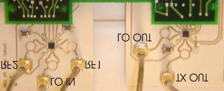
(图1 RX-Board（左）和 TX-Board（右）通过 IF-Hardware 连接到主板)

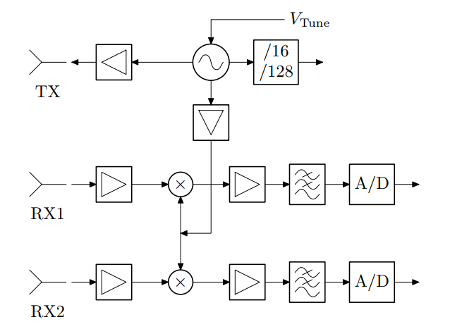
(图2 雷达系统框图)

2.FMCW雷达方程

In the following the equations for the FMCW Radar principle are presented in order to derive the implemented algorithms. The basic idea in FMCW is to generate a linear frequency ramp. The transmit frequency for one ramp with bandwidth B and duration T between [-T/2; T/2] can be expressed as:

下面给出了FMCW雷达原理的方程，以推导实现的算法。FMCW的基本思想是产生一个带宽为B，持续时间T为[-T/2，T/2]的线性调频信号，其发射频率可以表示为:

$f_{\mathrm{T}}(t)=f_{\mathrm{c}}+\frac{B}{T}t$（1）

The phase ϕT(t) of the transmitted signal cos (ϕT(t)) becomes after integration:

发射信号 cos (φT(t)) 的相位 φT(t) 积分后变为：

$\begin{array}{rl}{\phi }_{\mathrm{T}}(t)& =2\pi {\int }_{-T/2}^t{f}_{\mathrm{T}}(t)\mathrm{d}t\\ & ={2\pi \left(f_{\mathrm{c}}t+\frac{1}{2}\cdot \frac{B}{T}{t}^2\right)|}_{-T/2}^t\\ & =2\pi \left(f_{\mathrm{c}}t+\frac{1}{2}\cdot \frac{B}{T}{t}^2\right)-{\phi }_{T0}\end{array}$（2）

The phase of the downconverted signal Δϕ(t) = ϕT(t) -ϕT(t - τ) is:

下变频（混频）信号的相位Δϕ(t) = ϕT(t) -ϕT(t - τ) 为：

$\Delta \phi (t)=2\pi \left(f_{\mathrm{c}}\tau +\frac{B}{T}t\tau -\frac{B}{2T}{\tau }^2\right)$（3）

τ is the delay between the transmitted and received signal of one target. The last term in the equation above can be neglected because τ/T 1. For calculation of the delay τ = 2(R + v · t)/c a target at distance R with constant velocity v is assumed. This leads to:

τ 是一个目标的发射和接收信号之间的延迟。 上式中的最后一项可以忽略，因为 τ/T 远小于1。为了计算延迟 τ = 2(R + v · t)/c，假设目标距离为 R，速度为恒速 v。 这将出现：

$\Delta \phi (t)=2\pi \left[\frac{2f_{c}R}{c}+\left(\frac{2f_c\cdot v}{c}+\frac{2B\cdot R}{Tc}\right)t+\frac{2B\cdot v}{T\cdot c}{t}^2\right]$（4）

The last term is called Range-Doppler-Coupling and can be neglected again:

最后一项称为 Range-Doppler-Coupling（距离-多普勒耦合），可以再次忽略：

$\Delta \phi (t)=2\pi \left[\frac{2f_{c}R}{c}+\left(\frac{2f_c\cdot v}{c}+\frac{2B\cdot R}{Tc}\right)t\right]$（5）

The generated frequency is therefore:

因此产生的频率为:

$f_{\mathrm{I}\mathrm{F}}=\frac{2f_{\mathrm{c}}\cdot v}{c}+\frac{2B\cdot R}{Tc}$（6）

调皮哥笔记：这个就是要推导得到的中频信号的频率表达式，这个公式至关重要。

The received signal sIF = cos(Δϕ(t)) is sampled with an interval TA, the samples are multiplied with a window function w(n) and a zero padding is performed, before a Fast Fourier Transform with the resulting samples is done. The spectrum is symmetric, because the input signal is real. The complex baseband signal can be obtained by sIF(t) + i · H{sIF(t)}, where H{. . .} denotes the Hilbert transformation:

接收信号$s_{\mathrm{I}\mathrm{F}}=\cos (\Delta \phi (t))$ 用间隔 $T_{\mathrm{A}}$ 进行采样，采样与窗口函数w(n)相乘，并进行零填充，然后对得到的样本进行快速傅里叶变换,得到的频谱是对称的，因为输入信号是实数。复基带信号可由 s I F ( t ) + i ⋅ H { s I F ( t ) } s_{\mathrm{IF}}(t)+i \cdot H\left\{s_{\mathrm{IF}}(t)\right\} sIF​(t)+i⋅H{sIF​(t)} 得到，其中H{. .}表示希尔伯特变换:

$s_{\mathrm{B}}(n)=A\cdot w(n)e^{i\cdot 2\pi \left[\frac{2f_{\mathrm{C}}R}{c}+\left(\frac{2f_{\mathrm{c}}\cdot v}{c}+\frac{2B\cdot R}{Tc}\right)T_{\mathrm{A}}n\right]}$（7）

In order to simplify the following equations the window function isn’t taken into accout and A is set to one, which doesn’t cause the loss of generality.

为了简化后续的方程，不考虑窗函数，将A设为1，这样不会失去一般性。

3. 基于二维 FFT 的目标检测

For this algorithm, which has been described in [5], L frequency ramps have to be generated after another like shown in fig. 3. The ramp repetition intervall is called TRRI in the following.

对于该算法，已在 文献[5] 中进行了描述，L 个chirp斜坡必须依次生成，如图 3 所示。斜坡重复间隔以下称为TRRI。

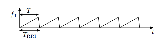
(图3 2D-FFT 的斜坡生成)

The resulting IF-Signal can be expressed as:

产生的 IF 信号可以表示为：

$s_{\mathrm{I}\mathrm{F},2\mathrm{D}}(t)={\sum }_{l=0}^{L-1}{e}^{i\cdot 2\pi \left[\frac{2f_c\left(R+v\cdot {\mathrm{T}}_{\mathrm{R}\mathrm{R}}\cdot l\right)}{c}+\left(\frac{2f_c\cdot v}{c}+\frac{2B\cdot \left(R+v{T}_{\mathrm{R}\mathrm{R}\mathrm{I}}\cdot l\right)}{Tc}\right)\cdot t\right]}$
$\cdot \mathrm{rect}\left(\frac{t-l\cdot T_{\mathrm{R}\mathrm{R}\mathrm{I}}}{T}\right)$（8）

The frequency increase can also be neglected, because the movement during the measurement is short compared to the distance R.

频率增加也可以忽略不计，因为与距离 R 相比，测量期间的移动很短（这里指忽略多普勒频移的变化的影响）。

$\begin{array}{rl}{s}_{\mathrm{I}\mathrm{F},2\mathrm{D}}(t)& =e^{i\cdot 4\pi f_{\mathrm{c}}\cdot R/c}\sum _{l=0}^{L-1}{e}^{i\cdot 2\pi [\frac{2f_{\mathrm{c}}\cdot v\cdot T_{\mathrm{R}\mathrm{R}\mathrm{I}}\cdot l}{c}}+\left(\frac{2f_{\mathrm{c}}\cdot v}{c}+\frac{2B\cdot R}{Tc}\right)\cdot t]\\ & \cdot \mathrm{rect}\left(\frac{t-l\cdot T_{\mathrm{R}\mathrm{R}\mathrm{I}}}{T}\right)\end{array}$（9）

The signal is sampled with fA = 1/TA during each ramp and a two dimensional fourier transformation is performed:

在每个斜坡期间以 fA = 1/TA 对信号进行采样，并执行二维傅立叶变换：

$S_{2\mathrm{D}}(k,p)=e^{i\cdot 4\pi f_c\cdot R/c}$
${\sum }_{l=0}^{L-1}{\sum }_{n=0}^{N-1}{e}^{i\cdot 4\pi \frac{v{T}_{\mathrm{R}\mathrm{R}\mathrm{L}}\cdot f_{\mathrm{C}}}{c}}l{e}^{i\cdot 2\pi \left[\left(\frac{2f_{\mathrm{C}}\cdot v}{c}+\frac{2B\cdot R}{Tc}\right)\cdot n\cdot T_A\right]}\cdot e^{-i\cdot 2\pi \left(\frac{l\cdot p}{LZ}+\frac{n\cdot k}{N_{\mathrm{Z}}}\right)}$（10）

NZ and LZ is the matrix size of S2D after zero-padding. Reordering the equation above leads to:

NZ 和 LZ 是补零后 S2D 的矩阵大小。 重新排序上面的等式导致：

$S_{2\mathrm{D}}(k,p)=e^{i\cdot 4\pi f_c\cdot R/c}$
${\sum }_{l=0}^{L-1}{e}^{i\cdot 4\pi \frac{v{T}_{\mathrm{R}\mathrm{R}\mathrm{R}}\cdot f_{\mathrm{c}}}{c}}l\left[{\sum }_{n=0}^{N-1}{e}^{i\cdot 2\pi \left[\left(\frac{2f_{\mathrm{C}}\cdot v}{c}+\frac{2B\cdot R}{Tc}\right)\cdot n\cdot T_A-\frac{n\cdot k}{N_{\mathrm{Z}}}\right]}\right]\cdot e^{\frac{-i\cdot 2\pi \cdot \cdot \cdot p}{L_{\mathrm{Z}}}}$（11）

From this equation it becomes obvious that a peak appears at the following position:

从这个等式可以明显看出，峰值出现在以下位置：

$k=\left(\frac{2f_{\mathrm{c}}\cdot v}{c}+\frac{2B\cdot R}{Tc}\right)T_{\mathrm{A}}\cdot N_{\mathrm{Z}}$
$p=\frac{2v\cdot f_{\mathrm{c}}\cdot T_{\mathrm{R}\mathrm{R}\mathrm{I}}\cdot L}{c}=f_{\mathrm{D}}\cdot T_{\mathrm{R}\mathrm{R}\mathrm{I}}\cdot L_{\mathrm{Z}}$（12和13）

In order to fulfill the sampling theorem, the following constraint for the maximum doppler frequency fD,max must be met:

为了满足采样定理，必须满足最大多普勒频率 $f_{\mathrm{D}},\max$ 的以下约束：

$f_{\mathrm{D},\max }<\frac{1}{2\cdot T_{\mathrm{R}\mathrm{R}\mathrm{I}}}(14)$（14）

It can be easily seen that the velocity resolution Δv is determined by the overall measurement time TRRI · L:

很容易看出，速度分辨率 $\Delta v$ 由总测量时间 $T_{\mathrm{R}\mathrm{R}\mathrm{I}}\cdot L$ 决定：

$\Delta v=\frac{c}{2f_c^f\cdot T_{\mathrm{R}\mathrm{R}\mathrm{I}}\cdot L}$（15）

The straight-forward way to implement the algorithm is to perform a FFT for each single ramp. For each rangegate the doppler spectrum must be calculated. The target detection can be done with a simple CFAR algorithm directly in the doppler spectrum, because the number of targets in one doppler spectrum is low in practical cases. For the prototype setup the following parameters have been chosen: Ramps L = 32, Ramp Duration T = 200μs, Ramp Repetition Intervall TRRI = 220μs, Sampling Frequency fA = 2.5 MHz. Therefore N = 500 = T · fA samples are generated per ramp. The samples are multiplied with a blackman window and after zero-padding to NZ = 1024 samples the FFT for each ramp is calculated. A measurement in the laboratory is depicted in fig. 4, where the displayed range is limited to 7 m.

实现该算法的直接方法是对每个chirp执行 FFT， 对于每个距离门必须计算多普勒频谱。 目标检测可以通过简单的 CFAR 算法直接在多普勒频谱中完成，因为在实际情况下，一个多普勒频谱中的目标数量很少。 对于原型设置，已选择以下参数：chirp个数 L = 32，斜坡持续时间 T = 200μs，斜坡重复间隔 TRRI = 220μs，采样频率 fA = 2.5 MHz。 因此，每个斜坡生成 N = 500 = T · fA 个采样点，并与布莱克曼窗口（blackman）相乘，在零填充到 NZ = 1024 个样本后，计算每个斜坡的 FFT。 实验室中的测量如图 4 所示，显示距离限制为 7 m。

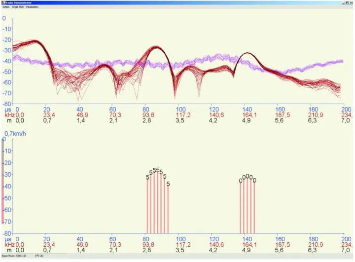
(图4 使用 2D-FFT 进行检测：3 m 处的移动目标，5 m 处的静态目标)

In the upper part the time domain signal and the logarithmic FFT amplitude of each ramp is shown, while the detected targets can be seen in the lower part. There’s the logarithmic amplitude of the doppler spectrum shown where the velocity is drawn at the top of each bin. The target detection was performed in the doppler spectrum with a Cell AveragingCFAR(see [2]) and local maxima search. For calculation of the doppler spectrum a blackman window was applied again and zero-padding to LZ = 128 was used.

上半部分显示了每个chirp的时域信号和对数 FFT 幅度，而下半部分显示了检测到的目标的多普勒频谱的对数幅度，其中速度绘制在每个坐标的顶部。 目标检测是在多普勒频谱中使用 Cell Averaging CFAR（CA-CFAR）（参见 [2]）和局部最大值搜索进行的。 为了计算多普勒频谱，再次应用布莱克曼窗并使用零填充到 LZ = 128。

This measurement has been done with a TX-Chip with an integrated divider of 128 and a subsequent external divider of 10. The resulting signal around 19 MHz becomes a LVTTL-Logic-Signal with the help of voltage comparator. The frequency of this signal can be easily determined by the used FPGA. The VCO frequency is directly set by a D/A-converter that sets the voltage at the Tune-Input of the VCO. The tuning law of the VCO is determined by setting a number of different voltages. After this static calibration a frequency ramp can be generated by calculating the values for the D/A-converter with the measured tuning law。

该测量是使用带有128集成分频器 和后续外部的 10分频器 的 TX 芯片完成的，在电压比较器的帮助下，产生的 19 MHz 左右的信号变为 LVTTL 逻辑信号。 该信号的频率可以很容易地由所使用的 FPGA 产生， VCO 频率由 D/A 转换器直接设置，该转换器设置 VCO 调谐输入端的电压。 VCO 的调谐规律是通过设置多个不同的电压来确定的。 在此静态校准之后，可以通过使用测量的调谐定律计算 D/A 转换器的值来生成频率斜坡。

4.不同斜率的后续斜坡检测（不同斜率的三角波）

This method uses slow ramps with different slopes like shown in fig. 5.

该方法使用具有不同斜率的慢速斜坡，如图 5所示。

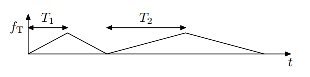
(图5 不同斜率的斜坡生成)

All Chirps occupy the bandwidth B. For the first up-chirp and down-chirp with ramp duration T1 the IFSignal is sampled with frequency fa,1 = 1/TA,1. The number of samples is therefore N = T1/TA,1 The sampling rate of the subsequent chirps with T2 is chosen according to the ramp duration:

所有chirp占用带宽B。对于第一个上行chirp和第一个下行chirp，坡道持续时间为T1, 中频信号的采样频率为 $f_{\mathrm{a},1}=1/T_{\mathrm{A},1}$ 。因此，采样点数 $N=T_1/T_{\mathrm{A},1}$ ，根据斜坡持续时间T2选择后续chirp 的采样率为:

$\frac{T_{\mathrm{A},1}}{T_{\mathrm{A},2}}=\frac{T_1}{T_2}=\frac{f_{\mathrm{A},2}}{f_{\mathrm{A},1}}=M$(16)

The Ratio M is an integer, e. g. M = 2. If the movement during the measurment time is small, one target creates the following frequencies for each ramp according to equ. 6:

比率M是一个整数，例如M = 2。如果在测量时间内目标的运动距离很小，一个目标根据公式6为每个chirp生成以下频率：

$\begin{array}{rl}{f}_{1,\text{ up }}& =\frac{2B\cdot R}{T_{1}c}+\frac{2f_{\mathrm{c}}\cdot v}{c}\\ f_{1,\text{ down }}& =\frac{2B\cdot R}{T_{1}c}-\frac{2f_{\mathrm{c}}\cdot v}{c}\\ f_{2,\text{ up }}& =\frac{2B\cdot R}{T_{2}c}+\frac{2f_{\mathrm{c}}\cdot v}{c}\\ f_{2,\text{ down }}& =\frac{2B\cdot R}{T_{2}c}-\frac{2f_{\mathrm{c}}\cdot v}{c}\end{array}$（17）

Taking equ. 11 into account, a peak around the following integer position in each FFT Spectrum occurs:

考虑到公式11，每个 FFT 频谱中以下整数位置附近出现峰值：

$\begin{array}{rl}{k}_{1,\text{ up }}& =\left[\frac{2B\cdot R}{c{T}_1}+\frac{2f_{\mathrm{c}}\cdot v}{c}\right]T_{\mathrm{A},1}\cdot N_{\mathrm{Z}}\\ k_{1,\text{ down }}& =\left[\frac{2B\cdot R}{c{T}_1}-\frac{2f_{\mathrm{c}}\cdot v}{c}\right]T_{\mathrm{A},1}\cdot N_{\mathrm{Z}}\\ k_{2,\text{ up }}& =\left[\frac{2B\cdot R}{c{T}_1\cdot M}+\frac{2f_{\mathrm{c}}\cdot v}{c}\right]T_{\mathrm{A},1}\cdot M\cdot N_{\mathrm{Z}}\\ k_{2,\text{ down }}& =\left[\frac{2B\cdot R}{c{T}_1\cdot M}-\frac{2f_{\mathrm{c}}\cdot v}{c}\right]T_{\mathrm{A},1}\cdot M\cdot N_{\mathrm{Z}}\end{array}$（18）

For each rangegate position in the FFT spectrum the corresponding discrete positions k1,down,k2,up and k2,down must be searched where the maximum velocity ±vmax must be covered. The following equation states the issue clearly, where xr and xv are the assumed range position and velocity increment:

对于 FFT 谱中的每个距离门位置 $k_{1,up}$ ，必须搜索相应的离散位置$k_{1,\text{ down }},k_{2,\text{ up }}$ 和 $k_2$, down ，其中必须覆盖最大速度 ±Vmax。 下面的等式清楚地说明了这个问题，其中 xr 和 xv 是假定的距离位置和速度增量：

$\begin{array}{rl}{k}_{1,\text{ up }}& =\left[\frac{R}{\Delta R}+\frac{v}{\Delta v}\right]\frac{N_{\mathrm{Z}}}{N}=x_r+x_v\\ k_{1,\text{ down }}& =\left[\frac{R}{\Delta R}-\frac{v}{\Delta v}\right]\frac{N_{\mathrm{Z}}}{N}=x_r-x_v\\ k_{2,\text{ up }}& =\left[\frac{R}{\Delta R}+\frac{v\cdot M}{\Delta v}\right]\frac{N_{\mathrm{Z}}}{N}=x_r+M\cdot x_v\\ k_{2,\text{ down }}& =\left[\frac{R}{\Delta R}-\frac{v\cdot M}{\Delta v}\right]\frac{N_{\mathrm{Z}}}{N}=x_r-M\cdot x_v\end{array}$（19）

The range resolution ΔR is determined by the bandwidth, Δv is the velocity resolution of the shortest ramp. After the FFT a CFAR is performed on each single ramp. Hence the search needs only to be done with the positions that have exceeded their CFAR threshold. So the calculation effort is quite relaxed. The exact implementation of the algorithm will be dependent of the used device, e.g. FPGA or DSP. Because there can be many peaks in one FFT spectrum, the CFAR-Algorithm must be of high quality which leads to the corresponding computional effort. The number of FFTs is low compared to the two dimensional method and equals the number of used ramps.

距离分辨率 ΔR 由带宽决定，Δv 是最短斜坡的速度分辨率。 在 FFT 之后，在每个斜坡上执行 CFAR。 因此，只需要对超过其 CFAR 阈值的位置进行搜索，所以计算工作相对简单。 算法的实现将取决于使用的设备，如 FPGA或DSP。 由于在一个 FFT 频谱中可能有许多峰，因此 CFAR 算法必须具有高质量，这会影响相应的计算工作量。 与二维方法相比，FFT 的数量较少，并且等于使用的斜坡的数量。

If one wants to use a fractional value instead of an integer value M, an interpolation in the spectrum can be done: A simple approach is to do a linear interpolation with the surrounding values under the constraint that the surrounding values are also greater than the CFAR threshold.

如果想用分数值代替整数值M，可以对频谱进行插值:一种简单的方法是对周围的值进行线性插值，约束条件是周围的值也大于CFAR阈值。

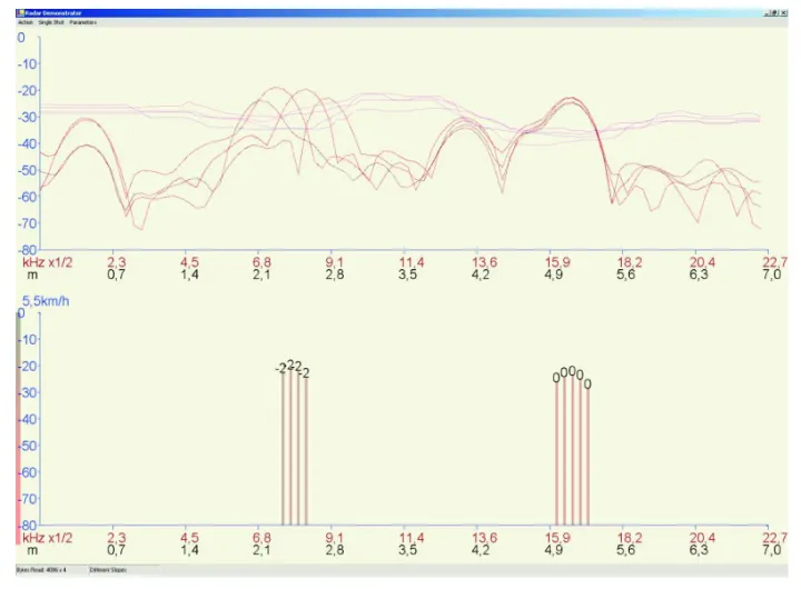
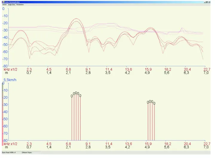
Fig. 6 and fig. 7 show a laboratory scene with a static and moving target. The logarithmic FFT amplitude and CFAR thresholds are depicted in the upper part, the lower part shows the detected targets. The separation of the peaks due to the doppler frequency can be clearly seen. The shown amplitude of the detected targets is the average of the amplitudes at the corresponding positions k1,up, k1,down, k2,up and k2,down.

图 6 和图 图 7 显示了具有静态和移动目标的实验室场景。 上半部分描绘了对数 FFT 幅度和 CFAR 阈值，下半部分显示了检测到的目标，可以清楚地看到由于多普勒频率导致的峰值分离（峰值不在同一个地方），检测到的目标的显示幅度是相应位置 k1,up, k1,down, k2,up 和 k2,down 的幅度的平均值。

(图6 不同斜率的检测：移动目标)

(图7 不同斜率的检测：静态目标)

The measurement parameters have been: Ramp Duration T1 = 2048 μs and T2 = 4096 μs, Sampling Rate fA,1 = 500 kHz and fA,1 = 250 kHz. The resulting N = 1024 samples per ramp are multiplied with a blackman window and a FFT is performed after zero-padding to NZ = 2048 Samples. An Ordered Statistics-CFAR is used for target detection on each ramp.

雷达的测量参数为：斜坡持续时间 T1 = 2048 μs 和 T2 = 4096 μs，采样率 fA,1 = 500 kHz 和 fA,1 = 250 kHz。 每个斜坡得到的 N = 1024 个样本与布莱克曼窗口相乘，并在零填充到 NZ = 2048 个样本后执行 FFT。 Ordered Statistics-CFAR（OS-CFAR） 用于每个斜坡上的目标检测。

With the presented algorithm the final targets are extracted under the additional constraint that the target positions are local maxima in the doppler range. For this measurement a TX-Chip with an integrated divider of 16 has been used, the divided VCO-Signal at 1.5 GHz is fed to a PLL Synthesizer whose reference signal is modulated to generate the desired frequency chirps. The algorithm can be generalised to an arbitrary number of ramps.

使用所提出的算法，可在目标位置是多普勒范围内的局部最大值的附加约束下提取最终目标。 对于此测量，使用了带有 16 分频器的 TX 芯片，1.5 GHz 的分频 VCO 信号被馈送到 PLL 合成器，其参考信号被调制以产生所需的chirp信号， 该算法可以推广到任意数量的斜坡。

The problem of range doppler detection has been addressed in [4] and [3] for FSCW-Radar(FS=Frequency Stepped) and FMCW and in [6] and [7] for FMCW. The problem of range doppler detection has been described as intersectioning process in the R-v-diagram (see equ. 17): Every beat frequency leads to a line in the R-v-diagram with different slope. For one target the intersection point of lines with different slopes must be searched. If there is an additional intersection, a ghost target is detected accidentally. This is especially a problem for distributed targets. The number of required targets to produce one ghost target is equal to the number of used ramps.

对于FSCW-Radar（FS=Frequency Stepped）和 FMCW的距离多普勒检测问题已经在文献 [4] 和 文献[3] 以及 [6] 和 [7] 中得到解决。 距离多普勒检测的问题已被描述为 R-V 图中的交叉过程（参见方程 17）：即 R-V 图中每个差拍频率会产生具有不同斜率的线。 对于一个目标，必须搜索具有不同斜率的线的交点，如果存在额外的交叉点，则会意外检测到虚假目标。 这对于分布式目标来说尤其是一个问题， 产生一个虚假目标所需的目标数量等于使用的斜坡数量。

5. 总结和展望

For the algorithm based on a two dimensional FFT fast ramps have to be generated to fulfill the sampling theorem for the highest doppler frequency. This leads to IF-Frequencies in the range of several megahertz. The ramp generation can be easily implemented with a D/A-converter that feeds the tune input of the VCO. The algorithm with different slopes requires slow ramps in order to achieve a certain velocity resolution. In that case the IF-frequencies are in the range of a few hundred kilohertz. The slow ramp generation allows the use of a Phase Locked Loop for ramp generation. In the future we want to implement the algorithms on an embedded device and test it in real traffic scenarios combined with angle detection according to the phase monopulse principle. The radar will also be tested with an improved version of the chipset which is currently under production.

对于基于二维 FFT 的算法，必须生成快速斜坡以满足最高多普勒频率的采样定理，这产生了了几兆赫兹范围内的中频频率。 斜坡生成可以通过一个 D/A 转换器轻松实现，该转换器为 VCO 的调谐输入提供数据。 不同坡度的算法需要较慢的坡道，以达到一定的速度分辨率，在这种情况下，中频频率在几百赫兹的范围内，缓慢的斜坡生成允许使用相位锁定环路来生成斜坡。未来我们将在嵌入式设备上实现该算法，并根据相位单脉冲原理结合角度检测在真实交通场景中进行测试，该雷达还将使用目前正在生产的改进版芯片组进行测试。

感谢阅读，感谢梨辣的分享！

6.参考文献

[1] Rohling H. Radar CFAR Thresholding in Clutter and Multiple Target Situations (IEEE Transactions on Aerospace and Electronic Systems, AES-19, July 1983,pp. 608-621)
[2] Ludloff A. Praxiswissen Radar und Radarsignalverarbeitung (Vieweg, 1998)
[3] Meinecke, Marc Michael; Rohling H. Combination of LFMCW and FSK Modulation Principles for Automotive Radar Systems (German Radar Symposium GRS 2000)
[4] Meinecke, Marc Michael; Rohling H. Waveform Design Principles for Automotive Radar Systems (German Radar Symposium GRS 2000)
[5] Stove, A.G.; Linear FMCW radar techniques (Radar and Signal Processing, IEE Proceedings F, Volume 139,Issue 5, Oct. 1992, pp.343-350)
[6] Folster, F.; Rohling H.; Lubbert U. An Automotive radar network based on 77GHz FMCW sensors (Radar Conference, 2005 IEEE International, 9-12 May 2005, pp. 871-876)
[7] Mende, R.; Rohling H.; A High-Performance AICC radar sensorconcept and results with an experimental vehicle (Radar 97(Conf. Publ. No. 449), 14.-16.Oct 1997, pp.21-25)