一、DCGAN介绍
DCGAN即使用卷积网络的对抗网络,其原理和GAN一样,只是把CNN卷积技术用于GAN模式的网络里,G(生成器)网在生成数据时,使用反卷积的重构技术来重构原始图片。D(判别器)网用卷积技术来识别图片特征,进而做出判别。同时,CDGAN中的卷积神经网络也做了一些结构的改变,以提高样本的质量和收敛速度。
DCGAN的generator网络结构图如下:

- G网中使用ReLU作为激活函数,最后一层使用Tanh作为激活函数。
- 去掉了FC层,使网络变为全卷积网络。
DCGAN的discriminator网络结构图如下:

- D中取消所有的池化层,使用转置卷积(transposed convolutional layer)并且步长大于等于2进行上采样。
- D网中也加入stride的卷积代替pooling。
- 在D网和G网中均使用批量归一化(batch normalization),而在最后一层时通常不会使用batch normalization,这是为了保证模型能够学习到数据的正确均值和方差。
- D网络中使用LeakyReLU作为激活函数。
- DCGAN中换成了两个卷积神经网络(CNN)的G和D,可以刚好的学习对输入图像层次化的表示,尤其在生成器部分会有更好的模拟效果。DCGAN在训练过程中会使用Adam优化算法。
三、网络实现
以人脸数据为例
1、环境配置(Environments)
- window10
- python3.6.4
- TensorFlow1.13.1
2、数据准备
数据集:face-swap
数据可以从网上自行下载,或者利用自己的数据,这里对数据的没有严格要求。我是采用了网络上的数据集,这里给出数据的下载地址:https://anonfile.com/p7w3m0d5be/face-swap.zip将解压的数据分别放入文件夹A和文件夹B
3、超参数设置(Hyper-Parameters)
- Image Size = 64x64
- Batch Size = 64
- Learning Rate = 0.00005
- Adam_beta1 = 0.5
- z_dim = 100
- Epoch = 500
# 导入需要的包
from PIL import Image  # Image 用于读取影像
#from skimage import io  # io也可用于读取影响,效果比Image读取的更好一些import tensorflow as tf  # 用于构建神经网络模型
import matplotlib.pyplot as plt  # 用于绘制生成影像的结果
import numpy as np  # 读取影像
import os  # 文件夹操作
import time  # 计时# 设置相关参数
is_training = True
input_dir = "./face/"  # 原始数据的文件夹路径# 设置超参数 hyper parameters
batch_size = 64
image_width = 64
image_height = 64
image_channel = 3
data_shape = [64, 64, 3]
data_length = 64 * 64 * 3z_dim = 100
learning_rate = 0.00005
beta1 = 0.5
epoch = 500
4、读取数据并将原始数据数据resize成64*64*3的格式,原始图像大小为256*256*3
# 读取数据的函数
def prepare_data(input_dir, floder):'''函数功能:通过输入图像的路径,读取训练数据:参数 input_dir: 图像数据所在的根目录,即"./face":参数 floder: 图像数据所在的子目录, 即"./face/A":return: 返回读取好的训练数据'''# 遍历图像路径,并获取图像数量images = os.listdir(input_dir + floder)image_len = len(images)# 设置一个空data,用于存放数据data = np.empty((image_len, image_width, image_height, image_channel), dtype="float32")# 逐个图像读取for i in range(image_len):# 如果导入的是skimage.io,则读取影像应该写为img = io.imread(input_dir + images[i])img = Image.open(input_dir + floder + "/" + images[i])  # 打开图像img = img.resize((image_width, image_height))  # 将256*256变成64*64arr = np.asarray(img, dtype="float32")  # 将格式改为np.arraydata[i, :, :, :] = arr  # 将其放入data中sess = tf.Session()sess.run(tf.initialize_all_variables())data = tf.reshape(data, [-1, image_width, image_height, image_channel])train_data = data * 1.0 / 127.5 - 1.0  # 对data进行正则化train_data = tf.reshape(train_data, [-1, data_length])  # 将其拉伸成一维向量train_set = sess.run(train_data)sess.close()return train_set
5、定义生成器函数
# 定义生成器
def Generator(z, is_training, reuse):'''函数功能:输入噪声z,生成图像gen_img:param z:即输入数据,一般为噪声:param is_training:是否为训练环节:return: 返回生成影像gen_img'''# 图像的channel维度变化为100->1024->512->256->128->3depths = [1024, 512, 256, 128] + [data_shape[2]]with tf.variable_scope("Generator", reuse=reuse):# 第一层100with tf.variable_scope("g_c1", reuse=reuse):output = tf.layers.dense(z, depths[0] * 4 * 4, trainable=is_training)output = tf.reshape(output, [batch_size, 4, 4, depths[0]])output = tf.nn.relu(tf.layers.batch_normalization(output, training=is_training))# 第二层反卷积层1024with tf.variable_scope("g_dc1", reuse=reuse):output = tf.layers.conv2d_transpose(output, depths[1], [5, 5], strides=(2, 2),padding="SAME", trainable=is_training)output = tf.nn.relu(tf.layers.batch_normalization(output, training=is_training))# 第三层反卷积层512with tf.variable_scope("g_dc2", reuse=reuse):output = tf.layers.conv2d_transpose(output, depths[2], [5, 5], strides=(2, 2),padding="SAME", trainable=is_training)output = tf.nn.relu(tf.layers.batch_normalization(output, training=is_training))# 第四层反卷积层256with tf.variable_scope("g_dc3", reuse=reuse):output = tf.layers.conv2d_transpose(output, depths[3], [5, 5], strides=(2, 2),padding="SAME", trainable=is_training)output = tf.nn.relu(tf.layers.batch_normalization(output, training=is_training))# 第五层反卷积层128with tf.variable_scope("g_dc4", reuse=reuse):output = tf.layers.conv2d_transpose(output, depths[4], [5, 5], strides=(2, 2),padding="SAME", trainable=is_training)gen_img = tf.nn.tanh(output)return gen_img
6、定义判别器函数
# 定义判别器
def Discriminator(x, is_training, reuse):'''函数功能:判别输入的图像是真或假:param x: 输入数据:param is_training: 是否为训练环节:return: 判别结果'''# 判别器的channel维度变化为:3->64->128->256->512depths = [data_shape[2]] + [64, 128, 256, 512]with tf.variable_scope("Discriminator", reuse=reuse):# 第一层卷积层,注意用的是leaky_relu函数with tf.variable_scope("d_cv1", reuse=reuse):output = tf.layers.conv2d(x, depths[1], [5, 5], strides=(2, 2),padding="SAME", trainable=is_training)output = tf.nn.leaky_relu(tf.layers.batch_normalization(output, training=is_training))# 第二层卷积层,注意用的是leaky_relu函数with tf.variable_scope("d_cv2", reuse=reuse):output = tf.layers.conv2d(output, depths[2], [5, 5], strides=(2, 2),padding="SAME", trainable=is_training)output = tf.nn.leaky_relu(tf.layers.batch_normalization(output, training=is_training))# 第三层卷积层,注意用的是leaky_relu函数with tf.variable_scope("d_cv3", reuse=reuse):output = tf.layers.conv2d(output, depths[3], [5, 5], strides=(2, 2),padding="SAME", trainable=is_training)output = tf.nn.leaky_relu(tf.layers.batch_normalization(output, training=is_training))# 第四层卷积层,注意用的是leaky_relu函数with tf.variable_scope("d_cv4", reuse=reuse):output = tf.layers.conv2d(output, depths[4], [5, 5], strides=(2, 2),padding="SAME", trainable=is_training)output = tf.nn.leaky_relu(tf.layers.batch_normalization(output, training=is_training))# 第五层全链接层with tf.variable_scope("d_c1", reuse=reuse):output = tf.layers.flatten(output)disc_img = tf.layers.dense(output, 1, trainable=is_training)return disc_img
7、编写保存结果
def plot_and_save(order, images):'''函数功能:绘制生成器的结果,并保存:param order::param images::return:'''# 将一个batch_size的所有图像进行保存batch_size = len(images)n = np.int(np.sqrt(batch_size))# 读取图像大小,并生成掩模canvasimage_size = np.shape(images)[2]n_channel = np.shape(images)[3]images = np.reshape(images, [-1, image_size, image_size, n_channel])canvas = np.empty((n * image_size, n * image_size, image_channel))# 为每个掩模赋值for i in range(n):for j in range(n):canvas[i * image_size:(i + 1) * image_size, j * image_size:(j + 1) * image_size, :] = images[n * i + j].reshape(64, 64, 3)# 绘制结果,并设置坐标轴plt.figure(figsize=(8, 8))plt.imshow(canvas, cmap="gray")label = "Epoch: {0}".format(order + 1)plt.xlabel(label)# 为每个文件命名if type(order) is str:file_name = orderelse:file_name = "face_gen" + str(order)# 保存绘制的结果plt.savefig(file_name)print(os.getcwd())print("Image saved in file: ", file_name)plt.close()8、定义训练过程
# 定义训练过程
def training():'''函数功能:实现DCGAN的训练过程'''# 准备数据。这里输入根目录,以A的影像为例进行图像生成data = prepare_data(input_dir, "A")# 构建网络结构,这是程序的核心部分---------------------------------------------x = tf.placeholder(tf.float32, shape=[None, data_length], name="Input_data")x_img = tf.reshape(x, [-1] + data_shape)z = tf.placeholder(tf.float32, shape=[None, z_dim], name="latent_var")G = Generator(z, is_training=True, reuse=False)D_fake_logits = Discriminator(G, is_training=True, reuse=False)D_true_logits = Discriminator(x_img, is_training=True, reuse=True)# 定义生成器的损失函数G_lossG_loss = tf.reduce_mean(tf.nn.sigmoid_cross_entropy_with_logits(logits=D_fake_logits, labels=tf.ones_like(D_fake_logits)))# 定义判别器的损失函数D_lossD_loss_1 = tf.reduce_mean(tf.nn.sigmoid_cross_entropy_with_logits(logits=D_true_logits, labels=tf.ones_like(D_true_logits)))D_loss_2 = tf.reduce_mean(tf.nn.sigmoid_cross_entropy_with_logits(logits=D_fake_logits, labels=tf.zeros_like(D_fake_logits)))D_loss = D_loss_1 + D_loss_2# 定义方差total_vars = tf.trainable_variables()d_vars = [var for var in total_vars if "d_" in var.name]g_vars = [var for var in total_vars if "g_" in var.name]# 定义优化方式with tf.control_dependencies(tf.get_collection(tf.GraphKeys.UPDATE_OPS)):g_optimization = tf.train.AdamOptimizer(learning_rate=learning_rate,beta1=beta1).minimize(G_loss, var_list=g_vars)d_optimization = tf.train.AdamOptimizer(learning_rate=learning_rate,beta1=beta1).minimize(D_loss, var_list=d_vars)print("we successfully make the network")# 网络模型构建结束------------------------------------------------------------# 训练模型初始化start_time = time.time()  # 计时sess = tf.Session()sess.run(tf.initialize_all_variables())# 逐个epoch训练for i in range(epoch):total_batch = int(len(data) / batch_size)d_value = 0g_value = 0# 逐个batch训练for j in range(total_batch):batch_xs = data[j * batch_size:j * batch_size + batch_size]# 训练判别器z_sampled1 = np.random.uniform(low=-1.0, high=1.0, size=[batch_size, z_dim])Op_d, d_ = sess.run([d_optimization, D_loss], feed_dict={x: batch_xs, z: z_sampled1})# 训练生成器z_sampled2 = np.random.uniform(low=-1.0, high=1.0, size=[batch_size, z_dim])Op_g, g_ = sess.run([g_optimization, G_loss], feed_dict={x: batch_xs, z: z_sampled2})# 尝试生成影像并保存images_generated = sess.run(G, feed_dict={z: z_sampled2})d_value += d_ / total_batchg_value += g_ / total_batchplot_and_save(i, images_generated)# 输出时间和损失函数losshour = int((time.time() - start_time) / 3600)min = int(((time.time() - start_time) - 3600 * hour) / 60)sec = int((time.time() - start_time) - 3600 * hour - 60 * min)print("Time: ", hour, "h", min, "min", sec, "sec", "   Epoch: ",i, "G_loss: ", g_value, "D_loss: ", d_value)
9、进行训练
if __name__ == "__main__":training()四、结果
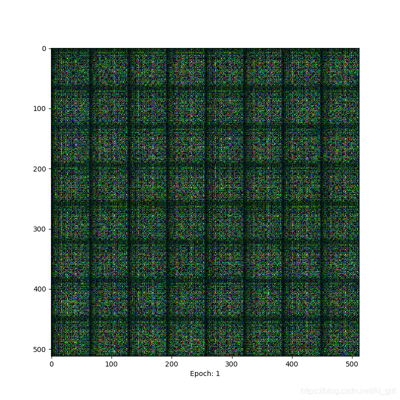
Epoch=1,基本什么也看不清
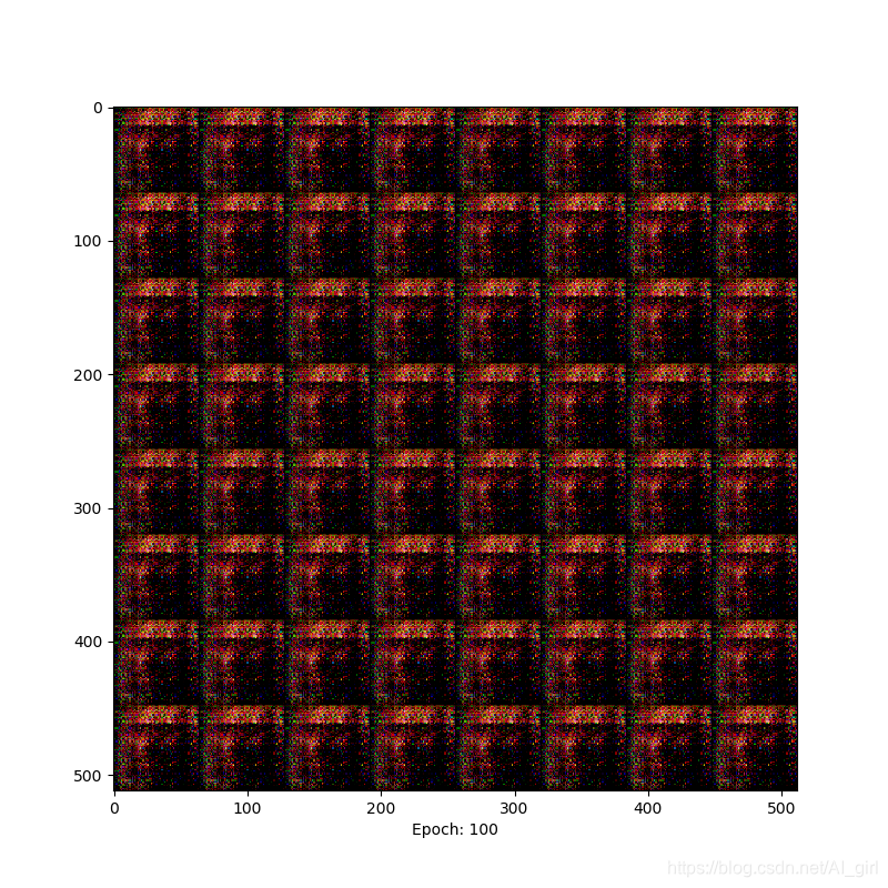
Epoch=100时,有了明显的纹理变化
Epoch=200时,能够明显的看到人脸轮廓

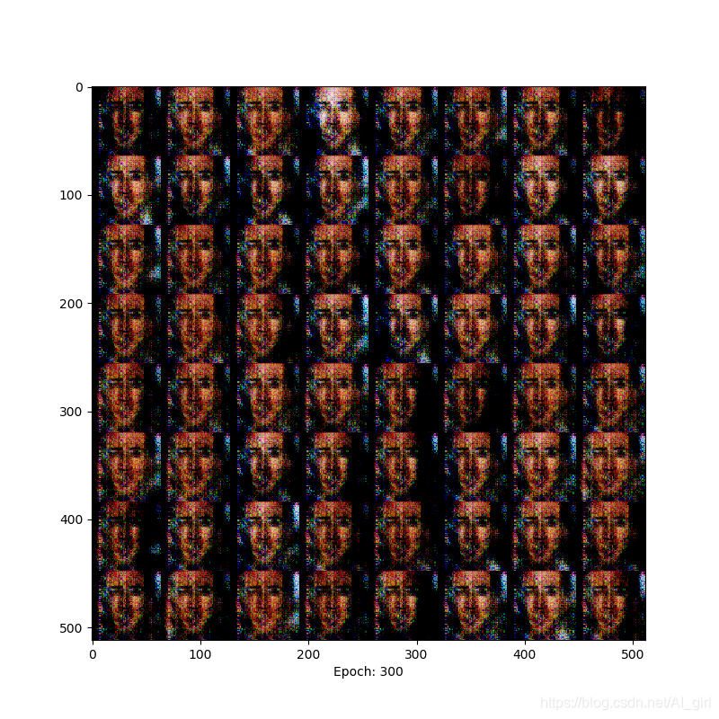
Epoch= 300时,面部特征比较清晰
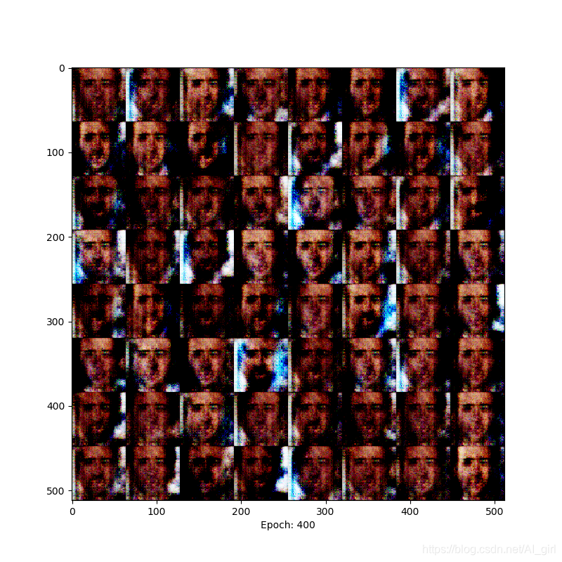
Epoch= 400时,人脸与背景区分明显
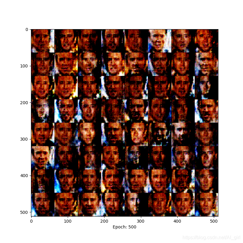
epoch= 500时,人脸色彩对比更加明显 ,已经能够清晰地辨别人脸。
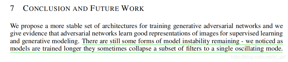
在训练的过程中出现了模型爆炸现象,这个问题在后期的WGAN中会得到解决。下面是从原文中截取的模型爆炸原因,原文地址请参考:https://arxiv.org/pdf/1511.06434.pdf
参考链接:
https://blog.csdn.net/z704630835/article/details/82254193
https://github.com/HyeongminLEE/Tensorflow_DCGAN