Skew(偏度)
在概率论和统计学中,偏度衡量实数随机变量概率分布的不对称性。偏度的值可以为正,可以为负或者甚至是无法定义。在数量上,偏度为负(负偏态)就意味着在概率密度函数左侧的尾部比右侧的长,绝大多数的值(包括中位数在内)位于平均值的右侧。偏度为正(正偏态)就意味着在概率密度函数右侧的尾部比左侧的长,绝大多数的值(但不一定包括中位数)位于平均值的左侧。偏度为零就表示数值相对均匀地分布在平均值的两侧,但不一定意味着其为对称分布。
import matplotlib.pyplot as pltplt.hist(test_scores_negative)
plt.show()plt.hist(test_scores_positive)
plt.show()plt.hist(test_scores_normal)
plt.show()from scipy.stats import skew
negative_skew = skew(test_scores_negative)
positive_skew = skew(test_scores_positive)
no_skew = skew(test_scores_normal)
'''
-0.6093247474592194
0.5376950498203763
0.0223645171350847
'''
- 图中描绘的是三个数据的直方图,表示了数据的分布,可以发现第一张图的数据大部分集中在平均值的右侧(负偏态),中间的图集中在平均值的左侧(正偏态),最后一张图集中在均值附近。
Kurtosis(峰度)
在统计学中,峰度(Kurtosis)衡量实数随机变量概率分布的峰态。峰度高就意味着方差增大是由低频度的大于或小于平均值的极端差值引起的。
峰度(Kurtosis)与偏态(Skewness)就是量测数据正态分布特性的两个指标。峰度衡量数据分布的平坦度(flatness)。尾部大的数据分布,其峰度值较大。正态分布的峰度值为3。偏态量度对称性。0说明是最完美的对称性,正态分布的偏态就是0。
- 峰度其公式如下:

- 偏态的计算公式如下:

kurt_platy = kurtosis(test_scores_platy)Modality(情态)
Modality refers to the number of modes, or peaks, in a distribution. Real-world data often is unimodal (only has one mode).
import matplotlib.pyplot as plt# This plot has one mode, making it unimodal
plt.hist(test_scores_uni)
plt.show()# This plot has two peaks, and is bimodal
# This could happen if one group of students learned the material, and one learned something else, for example.
plt.hist(test_scores_bi)
plt.show()# More than one peak means that the plot is multimodal
# We can't easily measure the modality of a plot, like we can with kurtosis or skew.
# Often, the best way to detect multimodality is to observe the plot.
plt.hist(test_scores_multi)
plt.show()
Mean(均值)
import matplotlib.pyplot as pltplt.hist(test_scores_normal)
# The axvline function will plot a vertical line over an existing plot
plt.axvline(test_scores_normal.mean())
plt.show()plt.hist(test_scores_negative)
plt.axvline(test_scores_negative.mean())
plt.show()plt.hist(test_scores_positive)
plt.axvline(test_scores_positive.mean())
plt.show()

Median(中位数)
- 同时显示中位数和均值
import numpy
import matplotlib.pyplot as plt# Plot the histogram
plt.hist(test_scores_negative)
# Compute the median
median = numpy.median(test_scores_negative)# Plot the median in blue (the color argument of "b" means blue)
plt.axvline(median, color="b")# Plot the mean in red
plt.axvline(test_scores_negative.mean(), color="r")# See how the median is further to the right than the mean?
# It's less sensitive to outliers, and isn't pulled to the left.
plt.show()
plt.hist(test_scores_positive)
plt.axvline(numpy.median(test_scores_positive), color="b")
plt.axvline(test_scores_positive.mean(), color="r")
plt.show()
- 下面的统计分析是基于NBA的数据集,大概格式如下
player,pos,age,bref_team_id,g,gs,mp,fg,fga,fg.,x3p,x3pa,x3p.,x2p,x2pa,x2p.,efg.,ft,fta,ft.,orb,drb,trb,ast,stl,blk,tov,pf,pts,season,season_end
[Quincy,Acy,SF,23,TOT,63,0,847,66,141,0.468,4,15,0.266666666666667,62,126,0.492063492063492,0.482,35,53,0.66,72,144,216,28,23,26,30,122,171,2013-2014,2013]
[Steven,Adams,C,20,OKC,81,20,1197,93,185,0.503,0,0,NA,93,185,0.502702702702703,0.503,79,136,0.581,142,190,332,43,40,57,71,203,265,2013-2014,2013]player – name of the player.
pts – the total number of points the player scored in the season.
ast – the total number of assists the player had in the season.
fg. – the player’s field goal percentage for the season.
Calculating Standard Deviation
- q其实std()函数就可以计算标准差
# The nba stats are loaded into the nba_stats variable.
def calc_column_deviation(column):mean = column.mean()variance = 0for p in column:difference = p - meansquare_difference = difference ** 2variance += square_differencevariance = variance / len(column)return variance ** (1/2)mp_dev = calc_column_deviation(nba_stats["mp"])
ast_dev = calc_column_deviation(nba_stats["ast"])
Normal Distribution
- norm.pdf可以将一组数据生成正态分布数据,给予每个数据相应的概率使得满足给定的均值方差。
import numpy as np
import matplotlib.pyplot as plt
# The norm module has a pdf function (pdf stands for probability density function)
from scipy.stats import norm# The arange function generates a numpy vector
# The vector below will start at -1, and go up to, but not including 1
# It will proceed in "steps" of .01.  So the first element will be -1, the second -.99, the third -.98, all the way up to .99.
points = np.arange(-1, 1, 0.01)# The norm.pdf function will take points vector and turn it into a probability vector
# Each element in the vector will correspond to the normal distribution (earlier elements and later element smaller, peak in the center)
# The distribution will be centered on 0, and will have a standard devation of .3
probabilities = norm.pdf(points, 0, .3)# Plot the points values on the x axis and the corresponding probabilities on the y axis
# See the bell curve?
plt.plot(points, probabilities)
plt.show()
points = np.arange(-10, 10, 0.1)
probabilities = norm.pdf(points, 0, 2)
plt.plot(points, probabilities)
plt.show()
Covariance(协方差)

# The nba_stats variable has been loaded.
def covariance(x, y):x_mean = sum(x) / len(x)y_mean = sum(y) / len(y)x_diffs = [i - x_mean for i in x]y_diffs = [i - y_mean for i in y]codeviates = [x_diffs[i] * y_diffs[i] for i in range(len(x))]return sum(codeviates) / len(codeviates)cov_stl_pf = covariance(nba_stats["stl"], nba_stats["pf"])
cov_fta_pts = covariance(nba_stats["fta"], nba_stats["pts"])
Correlations
- 相关性最常见的度量方法是Pearson’s r,也叫r-value.
from scipy.stats.stats import pearsonrr, p_value = pearsonr(nba_stats["fga"], nba_stats["pts"])
# As we can see, this is a very high positive r value -- close to 1
print(r)
r_fta_pts, p_value = pearsonr(nba_stats["fta"], nba_stats["pts"])
r_stl_pf, p_value = pearsonr(nba_stats["stl"], nba_stats["pf"])
'''
0.369861731248
'''
相关性的计算公式如下:

from numpy import cov
# The nba_stats variable has been loaded in.
r_fta_blk = cov(nba_stats["fta"], nba_stats["blk"])[0,1] / ((nba_stats["fta"].var() * nba_stats["blk"].var())** (1/2))
r_ast_stl = cov(nba_stats["ast"], nba_stats["stl"])[0,1] / ((nba_stats["ast"].var() * nba_stats["stl"].var())** (1/2))