faster-rcnn 之 RPN网络的结构解析以及RPN代码详解

【首先】：大家应该要了解卷积神经网络的连接方式，卷积核的维度，反向传播时是如何灵活的插入一层；这里我推荐一份资料，真是写的非常清晰，就是MatConvet的用户手册，这个框架底层借用的是caffe的算法，所以他们的数据结构，网络层的连接方式都是一样的；建议读者看看，很快的；

下载链接：点击打开链接

【前面5层】：作者RPN网络前面的5层借用的是ZF网络，这个网络的结构图我截个图放在下面，并分析下为什么是这样子的；

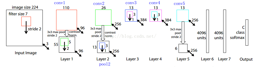
1、首先，输入图片大小是 224*224*3（这个3是三个通道，也就是RGB三种）

2、然后第一层的卷积核维度是 7*7*3*96 （所以大家要认识到卷积核都是4维的，在caffe的矩阵计算中都是这么实现的）；

3、所以conv1得到的结果是110*110*96 （这个110来自于 (224-7+pad)/2 +1 ，这个pad是我们常说的填充，也就是在图片的周围补充像素，这样做的目的是为了能够整除，除以2是因为2是图中的stride，这个计算方法在上面建议的文档中有说明与推导的）；

4、然后就是做一次池化，得到pool1，池化的核的大小是3*3，所以池化后图片的维度是55*55*96 （ (110-3+pad)/2 +1 =55 ）；

5、然后接着就是再一次卷积，这次的卷积核的维度是5*5*96*256 ，得到conv2：26*26*256；

6、后面就是类似的过程了，我就不详细一步步算了，要注意有些地方除法除不尽，作者是做了填充了，在caffe的prototxt文件中，可以看到每一层的pad的大小；

7、最后作者取的是conv5的输出，也就是13*13*256送给RPN网络的；

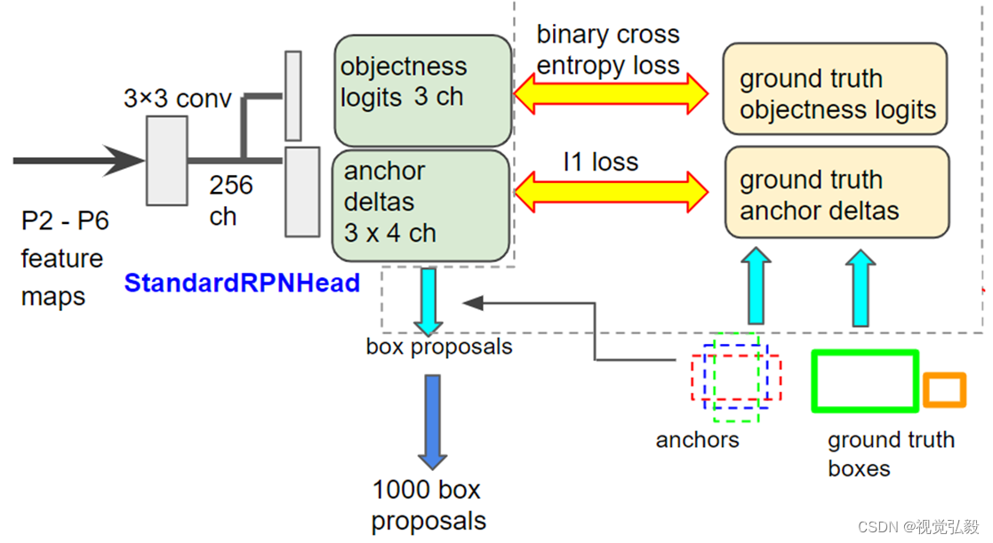
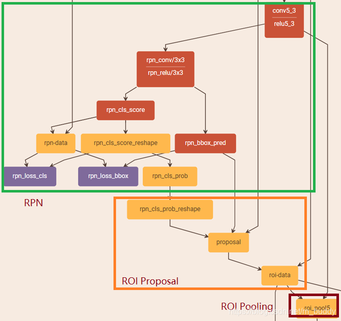
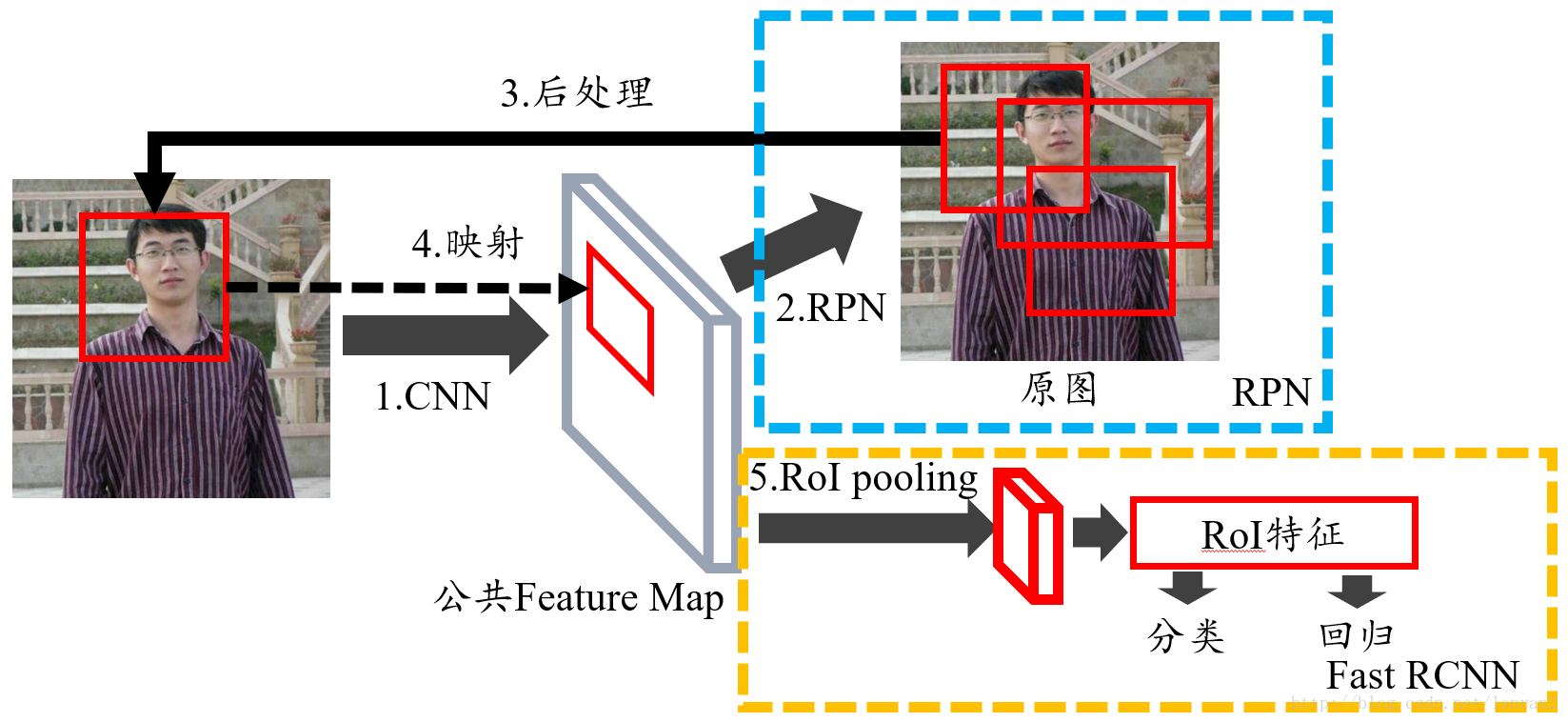
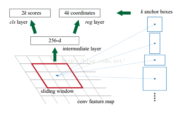
【RPN部分】：然后，我们看看RPN部分的结构：

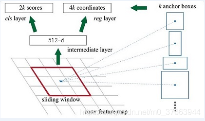
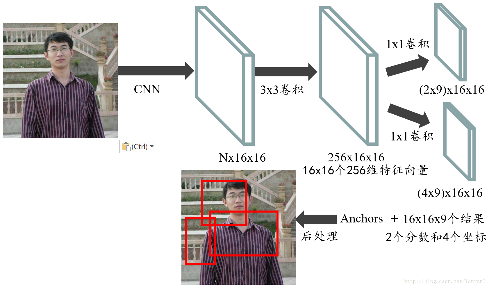
1、前面我们指出，这个conv feature map的维度是13*13*256的；

2、作者在文章中指出，sliding window的大小是3*3的，那么如何得到这个256-d的向量呢？这个很简单了，我们只需要一个3*3*256*256这样的一个4维的卷积核，就可以将每一个3*3的sliding window 卷积成一个256维的向量；

这里读者要注意啊，作者这里画的示意图仅仅是针对一个sliding window的；在实际实现中，我们有很多个sliding window，所以得到的并不是一维的256-d向量，实际上还是一个3维的矩阵数据结构；可能写成for循环做sliding window大家会比较清楚，当用矩阵运算的时候，会稍微绕些；

3、然后就是k=9，所以cls layer就是18个输出节点了，那么在256-d和cls layer之间使用一个1*1*256*18的卷积核，就可以得到cls layer，当然这个1*1*256*18的卷积核就是大家平常理解的全连接；所以全连接只是卷积操作的一种特殊情况（当卷积核的大小是1*1的时候）；

4、reg layer也是一样了，reg layer的输出是36个，所以对应的卷积核是1*1*256*36，这样就可以得到reg layer的输出了；

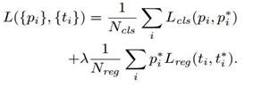
5、然后cls layer 和reg layer后面都会接到自己的损失函数上，给出损失函数的值，同时会根据求导的结果，给出反向传播的数据，这个过程读者还是参考上面给的文档，写的挺清楚的；

【作者关于RPN网络的具体定义】：这个作者是放在./models/pascal_voc/ZF/faster_rcnn_alt_opt/stage1_rpn_train.pt 文件中的；

我把这个文件拿出来给注释下：

[plain] view plain copy

name: "ZF"
layer {
name: 'input-data' #这一层就是最开始数据输入
type: 'Python'
top: 'data' # top表示该层的输出，所以可以看到这一层输出三组数据，data，真值框gt_boxes，和相关信息im_info
top: 'im_info' # 这些都是存储在矩阵中的
top: 'gt_boxes'
python_param {
module: 'roi_data_layer.layer'
layer: 'RoIDataLayer'
param_str: "'num_classes': 21"
}
}
#========= conv1-conv5 ============
layer {
name: "conv1"
type: "Convolution"
bottom: "data" # 输入data
top: "conv1" # 输出conv1，这里conv1就代表了这一层输出数据的名称，存储在对应的矩阵中
param { lr_mult: 1.0 }
param { lr_mult: 2.0 }
convolution_param {
num_output: 96
kernel_size: 7
pad: 3 # 这里可以看到卷积1层填充了3个像素
stride: 2
}
}
layer {
name: "relu1"
type: "ReLU"
bottom: "conv1"
top: "conv1"
}
layer {
name: "norm1"
type: "LRN"
bottom: "conv1"
top: "norm1" # 做归一化操作，通俗点说就是做个除法
lrn_param {
local_size: 3
alpha: 0.00005
beta: 0.75
norm_region: WITHIN_CHANNEL
engine: CAFFE
}
}
layer {
name: "pool1"
type: "Pooling"
bottom: "norm1"
top: "pool1"
pooling_param {
kernel_size: 3
stride: 2
pad: 1 # 池化的时候，又做了填充
pool: MAX
}
}
layer {
name: "conv2"
type: "Convolution"
bottom: "pool1"
top: "conv2"
param { lr_mult: 1.0 }
param { lr_mult: 2.0 }
convolution_param {
num_output: 256
kernel_size: 5
pad: 2
stride: 2
}
}
layer {
name: "relu2"
type: "ReLU"
bottom: "conv2"
top: "conv2"
}
layer {
name: "norm2"
type: "LRN"
bottom: "conv2"
top: "norm2"
lrn_param {
local_size: 3
alpha: 0.00005
beta: 0.75
norm_region: WITHIN_CHANNEL
engine: CAFFE
}
}
layer {
name: "pool2"
type: "Pooling"
bottom: "norm2"
top: "pool2"
pooling_param {
kernel_size: 3
stride: 2
pad: 1
pool: MAX
}
}
layer {
name: "conv3"
type: "Convolution"
bottom: "pool2"
top: "conv3"
param { lr_mult: 1.0 }
param { lr_mult: 2.0 }
convolution_param {
num_output: 384
kernel_size: 3
pad: 1
stride: 1
}
}
layer {
name: "relu3"
type: "ReLU"
bottom: "conv3"
top: "conv3"
}
layer {
name: "conv4"
type: "Convolution"
bottom: "conv3"
top: "conv4"
param { lr_mult: 1.0 }
param { lr_mult: 2.0 }
convolution_param {
num_output: 384
kernel_size: 3
pad: 1
stride: 1
}
}
layer {
name: "relu4"
type: "ReLU"
bottom: "conv4"
top: "conv4"
}
layer {
name: "conv5"
type: "Convolution"
bottom: "conv4"
top: "conv5"
param { lr_mult: 1.0 }
param { lr_mult: 2.0 }
convolution_param {
num_output: 256
kernel_size: 3
pad: 1
stride: 1
}
}
layer {
name: "relu5"
type: "ReLU"
bottom: "conv5"
top: "conv5"
}
#========= RPN ============
# 到我们的RPN网络部分了，前面的都是共享的5层卷积层的部分
layer {
name: "rpn_conv1"
type: "Convolution"
bottom: "conv5"
top: "rpn_conv1"
param { lr_mult: 1.0 }
param { lr_mult: 2.0 }
convolution_param {
num_output: 256
kernel_size: 3 pad: 1 stride: 1 #这里作者把每个滑窗3*3，通过3*3*256*256的卷积核输出256维，完整的输出其实是12*12*256,
weight_filler { type: "gaussian" std: 0.01 }
bias_filler { type: "constant" value: 0 }
}
}
layer {
name: "rpn_relu1"
type: "ReLU"
bottom: "rpn_conv1"
top: "rpn_conv1"
}
layer {
name: "rpn_cls_score"
type: "Convolution"
bottom: "rpn_conv1"
top: "rpn_cls_score"
param { lr_mult: 1.0 }
param { lr_mult: 2.0 }
convolution_param {
num_output: 18 # 2(bg/fg) * 9(anchors)
kernel_size: 1 pad: 0 stride: 1 #这里看的很清楚，作者通过1*1*256*18的卷积核，将前面的256维数据转换成了18个输出
weight_filler { type: "gaussian" std: 0.01 }
bias_filler { type: "constant" value: 0 }
}
}
layer {
name: "rpn_bbox_pred"
type: "Convolution"
bottom: "rpn_conv1"
top: "rpn_bbox_pred"
param { lr_mult: 1.0 }
param { lr_mult: 2.0 }
convolution_param {
num_output: 36 # 4 * 9(anchors)
kernel_size: 1 pad: 0 stride: 1 <span style="font-family: Arial, Helvetica, sans-serif;">#这里看的很清楚，作者通过1*1*256*36的卷积核，将前面的256维数据转换成了36个输出</span>
weight_filler { type: "gaussian" std: 0.01 }
bias_filler { type: "constant" value: 0 }
}
}
layer {
bottom: "rpn_cls_score"
top: "rpn_cls_score_reshape" # 我们之前说过，其实这一层是12*12*256的，所以后面我们要送给损失函数，需要将这个矩阵reshape一下，我们需要的是144个滑窗，每个对应的256的向量
name: "rpn_cls_score_reshape"
type: "Reshape"
reshape_param { shape { dim: 0 dim: 2 dim: -1 dim: 0 } }
}
layer {
name: 'rpn-data'
type: 'Python'
bottom: 'rpn_cls_score'
bottom: 'gt_boxes'
bottom: 'im_info'
bottom: 'data'
top: 'rpn_labels'
top: 'rpn_bbox_targets'
top: 'rpn_bbox_inside_weights'
top: 'rpn_bbox_outside_weights'
python_param {
module: 'rpn.anchor_target_layer'
layer: 'AnchorTargetLayer'
param_str: "'feat_stride': 16"
}
}
layer {
name: "rpn_loss_cls"
type: "SoftmaxWithLoss" # 很明显这里是计算softmax的损失，输入labels和cls layer的18个输出（中间reshape了一下），输出损失函数的具体值
bottom: "rpn_cls_score_reshape"
bottom: "rpn_labels"
propagate_down: 1
propagate_down: 0
top: "rpn_cls_loss"
loss_weight: 1
loss_param {
ignore_label: -1
normalize: true
}
}
layer {
name: "rpn_loss_bbox"
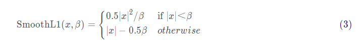
type: "SmoothL1Loss" # 这里计算的框回归损失函数具体的值
bottom: "rpn_bbox_pred"
bottom: "rpn_bbox_targets"
bottom: "rpn_bbox_inside_weights"
bottom: "rpn_bbox_outside_weights"
top: "rpn_loss_bbox"
loss_weight: 1
smooth_l1_loss_param { sigma: 3.0 }
}
#========= RCNN ============
# Dummy layers so that initial parameters are saved into the output net
layer {
name: "dummy_roi_pool_conv5"
type: "DummyData"
top: "dummy_roi_pool_conv5"
dummy_data_param {
shape { dim: 1 dim: 9216 }
data_filler { type: "gaussian" std: 0.01 }
}
}
layer {
name: "fc6"
type: "InnerProduct"
bottom: "dummy_roi_pool_conv5"
top: "fc6"
param { lr_mult: 0 decay_mult: 0 }
param { lr_mult: 0 decay_mult: 0 }
inner_product_param {
num_output: 4096
}
}
layer {
name: "relu6"
type: "ReLU"
bottom: "fc6"
top: "fc6"
}
layer {
name: "fc7"
type: "InnerProduct"
bottom: "fc6"
top: "fc7"
param { lr_mult: 0 decay_mult: 0 }
param { lr_mult: 0 decay_mult: 0 }
inner_product_param {
num_output: 4096
}
}
layer {
name: "silence_fc7"
type: "Silence"
bottom: "fc7"
}

anchors作为产生proposal的rpn中的一个重点内容，在Faster R-CNN中被重点介绍，下面我们来学习一下anchors产生部分代码。我主要将其中的部分重点代码展示出来。代码引用自Shaoqing Ren的Matlab下Faster R-CNN。

首先在Faster R-CNN迭代rpn和Fast R-CNN部分训练的前面，有一个产生anchors 的函数，我们称其产生的为base anchor，函数如下：

function anchors = proposal_generate_anchors(cache_name, varargin)
% anchors = proposal_generate_anchors(cache_name, varargin)
% --------------------------------------------------------
% Faster R-CNN
% Copyright (c) 2015, Shaoqing Ren
% Licensed under The MIT License [see LICENSE for details]
% --------------------------------------------------------%% inputsip = inputParser;ip.addRequired('cache_name',                        @isstr);% the size of the base anchor ip.addParamValue('base_size',       16,             @isscalar);% ratio list of anchorsip.addParamValue('ratios',          [0.5, 1, 2],    @ismatrix);% scale list of anchorsip.addParamValue('scales',          2.^[3:5],       @ismatrix);    ip.addParamValue('ignore_cache',    false,          @islogical);ip.parse(cache_name, varargin{:});opts = ip.Results;%%if ~opts.ignore_cacheanchor_cache_dir            = fullfile(pwd, 'output', 'rpn_cachedir', cache_name); mkdir_if_missing(anchor_cache_dir);anchor_cache_file           = fullfile(anchor_cache_dir, 'anchors');endtryld                      = load(anchor_cache_file);anchors                 = ld.anchors;catchbase_anchor             = [1, 1, opts.base_size, opts.base_size];% 围绕[base_anchor]随机ratios抖动ratio_anchors           = ratio_jitter(base_anchor, opts.ratios);% 围绕[base_anchor]随机scales抖动anchors                 = cellfun(@(x) scale_jitter(x, opts.scales), num2cell(ratio_anchors, 2), 'UniformOutput', false);anchors                 = cat(1, anchors{:});if ~opts.ignore_cachesave(anchor_cache_file, 'anchors');endendend
% 具体ratio_jitter，scale_jitter函数请关注原代码1
2
3
4
5
6
7
8
9
10
11
12
13
14
15
16
17
18
19
20
21
22
23
24
25
26
27
28
29
30
31
32
33
34
35
36
37
38
39
40
41
42
43
44
45
1
2
3
4
5
6
7
8
9
10
11
12
13
14
15
16
17
18
19
20
21
22
23
24
25
26
27
28
29
30
31
32
33
34
35
36
37
38
39
40
41
42
43
44
45

我在实验过程中设置断点，截取自己生成的anchor数值作为例子，如下：

anchor：9*4
[   -83     -39     100    56    ]
[   -175    -87     192    104   ]
[   -359    -183    376    200   ]
[   -55     -55     72     72    ]
[   -119    -119    136    136   ]
[   -247    -247    264    264   ]
[   -35     -79     52     96    ]
[   -79     -167    96     184   ]
[   -167    -343    184    360   ]1
2
3
4
5
6
7
8
9
10
1
2
3
4
5
6
7
8
9
10

可以看出，生成的9个anchor，前三排基本除去一些随机抖动以外不同scale但是ratio相同，均为[-2, -1, 2, 1]，中间三排为[-1, -1, 1, 1]，最后三排为[-1, -2, 1, 2]。
根据文章，这里即文章所说的9中anchor，即base anchor。

在rpn训练的过程中，针对每一张样本图像的大小与网络，得到所有anchor。

function [anchors, im_scales] = proposal_locate_anchors(conf, im_size, target_scale, feature_map_size)
% [anchors, im_scales] = proposal_locate_anchors(conf, im_size, target_scale, feature_map_size)
% --------------------------------------------------------
% Faster R-CNN
% Copyright (c) 2015, Shaoqing Ren
% Licensed under The MIT License [see LICENSE for details]
% --------------------------------------------------------   
% generate anchors for each scale% only for fcnif ~exist('feature_map_size', 'var')feature_map_size = [];endfunc = @proposal_locate_anchors_single_scale;if exist('target_scale', 'var')[anchors, im_scales] = func(im_size, conf, target_scale, feature_map_size);else[anchors, im_scales] = arrayfun(@(x) func(im_size, conf, x, feature_map_size), ...conf.scales, 'UniformOutput', false);endendfunction [anchors, im_scale] = proposal_locate_anchors_single_scale(im_size, conf, target_scale, feature_map_size)if isempty(feature_map_size)im_scale = prep_im_for_blob_size(im_size, target_scale, conf.max_size);img_size = round(im_size * im_scale);% 没有特征图时候，基于前面计算出的output高和宽，计算output_sizeoutput_size = cell2mat([conf.output_height_map.values({img_size(1)}), conf.output_width_map.values({img_size(2)})]);else%有特征图时候，直接赋值给output_sizeim_scale = prep_im_for_blob_size(im_size, target_scale, conf.max_size);output_size = feature_map_size;end% 针对output的高和宽，产生shift_x，shift_y。% shift_x大小为1*output列数shift_x = [0:(output_size(2)-1)] * conf.feat_stride;% shift_y大小为1*output行数shift_y = [0:(output_size(1)-1)] * conf.feat_stride;[shift_x, shift_y] = meshgrid(shift_x, shift_y);% concat anchors as [channel, height, width], where channel is the fastest dimension.% 这里意思就是对应output每一个像素处，根据conf.anchors（即前面提到的生成的base anchors）产生一系列anchorsanchors = reshape(bsxfun(@plus, permute(conf.anchors, [1, 3, 2]), ...permute([shift_x(:), shift_y(:), shift_x(:), shift_y(:)], [3, 1, 2])), [], 4);%   equals to  
%     anchors = arrayfun(@(x, y) single(bsxfun(@plus, conf.anchors, [x, y, x, y])), shift_x, shift_y, 'UniformOutput', false);
%     anchors = reshape(anchors, [], 1);
%     anchors = cat(1, anchors{:});end