Faster RCNN 中的RPN解析
文章目录
- Faster RCNN 中的RPN解析
- Anchor
- 分类
- bounding box regression
- proposal
- 参考
RCNN和Fast RCNN中使用Selective Search方法找出所有的候选框,SS方法非常耗时。Faster RCNN中提出RPN(region proposal network)替代SS方法提取候选框,并提出anchor的概念。虽然目前anchor free的各种算法层出不穷,但是anchor的思想也曾引领风潮。
RPN是一个轻量级的网络,仅仅包含一个33的卷积,11的分类层和1*1的回归层。RPN中引入了anchor的概念,每一个anchor要分positive和negative标签,所以分类分支将有2k个输出,每个anchor以 ( x , y , w , h ) \left( x, y, w, h \right) (x,y,w,h)表示坐标位置,回归分支将有4k个输出。

下图来自于py-faster-rcnn/models/pascal_voc/VGG16/faster_rcnn_end2end/test.prototxt中的RPN部分。

Anchor
RPN网络简单,但是刚入门时,有些不好理解,其中最难的地方在于anchor。anchor介绍见Faster RCNN中的Anchor
分类
在分类分支,由于anchor有背景和前景(bg/fg)之分,所有输出channels为2* 9=18,按照caffe的blob的格式,rpn_cls_score的输出格式为[batchsize, 18, H, W]。做softmax计算时,当axis=1,且预测大小为 (N, C, H, W)时,要求labels的数量为NHW。
分析:假设conv5_3的特征图形状为[N, C, H, W],经过一个33滑动窗口之后,输出大小为[N, 256, H, W],后又接一个11卷积的分类层,输出大小为[N, 2k, H, W]。对于大小为[H, W]的特征图,其生成的anchors数量为 H ∗ W ∗ k H*W*k H∗W∗k,所以总label 数量为HW*k。因此softmax运算时需要reshape一些,后再reshape恢复原状。
layer {name: "rpn_cls_score"type: "Convolution"bottom: "rpn/output"top: "rpn_cls_score"param { lr_mult: 1.0 decay_mult: 1.0 }param { lr_mult: 2.0 decay_mult: 0 }convolution_param {num_output: 18   # 2(bg/fg) * 9(anchors)kernel_size: 1 pad: 0 stride: 1weight_filler { type: "gaussian" std: 0.01 }bias_filler { type: "constant" value: 0 }}
}
layer {bottom: "rpn_cls_score"top: "rpn_cls_score_reshape"name: "rpn_cls_score_reshape"type: "Reshape"reshape_param { shape { dim: 0 dim: 2 dim: -1 dim: 0 } }
}
layer {name: "rpn_cls_prob"type: "Softmax"bottom: "rpn_cls_score_reshape"top: "rpn_cls_prob"
}
layer {name: 'rpn_cls_prob_reshape'type: 'Reshape'bottom: 'rpn_cls_prob'top: 'rpn_cls_prob_reshape'reshape_param { shape { dim: 0 dim: 18 dim: -1 dim: 0 } }
}
bounding box regression

bboxes通常以四维向量 ( x , y , w , h ) \left( x, y, w, h \right) (x,y,w,h)表示, ( x , y ) \left( x, y \right) (x,y)是一个bbox的中心点坐标, ( w , h ) \left( w, h \right) (w,h)为一个bbox的宽和高。如上图所示,假设红色矩形 P P P为Proposal box,绿色的框 G G G为ground-truth box。那么我们希望 P P P能够经过函数映射得到一个和 G G G更接近的回归框框 G ^ \hat{G} G^,如上图蓝色矩形。
用数学公式描述就是:给定 ( P x , P y , P w , P h ) \left( P_{x}, P_{y}, P_{w}, P_{h} \right) (Px,Py,Pw,Ph),寻找一映射 f f f,使得 f ( P x , P y , P w , P h ) = ( G ^ x , G ^ y , G ^ w , G ^ h ) f\left( P_{x}, P_{y}, P_{w}, P_{h} \right) = \left( \hat{G}_{x}, \hat{G}_{y}, \hat{G}_{w}, \hat{G}_{h} \right) f(Px,Py,Pw,Ph)=(G^x,G^y,G^w,G^h)且 ( G ^ x , G ^ y , G ^ w , G ^ h ) ≈ ( G x , G y , G w , G h ) \left(\hat{G}_{x}, \hat{G}_{y}, \hat{G}_{w}, \hat{G}_{h} \right) \approx \left(G_{x}, G_{y}, G_{w}, G_{h} \right) (G^x,G^y,G^w,G^h)≈(Gx,Gy,Gw,Gh)
解决方案:先平移,后尺度缩放。
- 先平移,将 P P P的中线点平移到 G G G的中心点,假设平移量为 ( Δ x , Δ y ) \left( \Delta x, \Delta y \right) (Δx,Δy), Δ x = w d x ( P ) , Δ y = P h d y ( P ) \Delta x = _{w}d_{x}\left( P \right) , \Delta y = P_{h}d_{y}\left( P \right) Δx=wdx(P),Δy=Phdy(P)
- 后尺度缩放 ( S w , S h ) \left( S_{w} , S_{h} \right) (Sw,Sh)
G ^ x = P w d x ( P ) + P x G ^ y = P h d y ( P ) + P y G ^ x = P w e x p ( d w ( P ) ) G ^ h = P h e x p ( d h ( P ) ) \begin{matrix} \hat{G}_{x} = P_{w}d_{x}\left( P \right) + P_{x} \\ \hat{G}_{y} = P_{h}d_{y}\left( P \right) + P_{y} \\ \hat{G}_{x} = P_{w} exp\left( d_{w} \left( P \right) \right) \\ \hat{G}_{h} = P_{h} exp\left( d_{h} \left( P \right) \right) \end{matrix} G^x=Pwdx(P)+PxG^y=Phdy(P)+PyG^x=Pwexp(dw(P))G^h=Phexp(dh(P))
通过学习这四个函数 d x ( P ) , d y ( P ) , d w ( P ) , d h ( P ) d_{x}\left( P \right) , d_{y}\left( P \right), d_{w} \left( P \right), d_{h} \left( P \right) dx(P),dy(P),dw(P),dh(P),我们就可以将proposal bbox P P P转化成为一个预测的ground-truth box G ^ \hat{G} G^.
将学习的函数统记为 d ∗ ( P ) , ∗ ∈ { x , y , h , w } d_{*}\left( P \right), * \in \left \{ x, y, h, w\right \} d∗(P),∗∈{x,y,h,w}。在RCNN中当 P P P和 G G G之间的 I o U > 0.6 IoU > 0.6 IoU>0.6时,可以将 d ∗ ( P ) d_{*}\left( P \right) d∗(P)看做一种线性变换,那么我们就可以用线性回归来建模。(在generate target anchor时,认定正样本的一项因素是 I o U > 0.7 IoU > 0.7 IoU>0.7。 d ∗ ( P ) d_{*}\left(P\right) d∗(P)是backbone最后一池化层特征( p o o l 5 pool_5 pool5)的线性函数,表示为 d ∗ ( P ) = w ∗ T ∅ 5 ( P ) d_{*} \left( P \right) = w_{*}^{T} \varnothing_{5} \left( P \right) d∗(P)=w∗T∅5(P),其中 w ∗ w_{*} w∗是学习到的参数向量,可以通过优化正则最小二乘法目标函数学习得到。
w ∗ = a r g m i n w ^ ∗ ∑ i N ( t ∗ i − w ^ ∗ T ∅ 5 ( P i ) ) 2 + λ ∥ w ^ x ∥ 2 w_{*} = argmin_{\hat{w}_{*}} \sum_{i}^{N} \left( t_{*}^{i} - \hat{w}_{*}^{T} \varnothing_{5}\left ( P^{i} \right ) \right) ^{2} + \lambda \left \| \hat{w}_{x} \right \| ^{2} w∗=argminw^∗i∑N(t∗i−w^∗T∅5(Pi))2+λ∥w^x∥2
其中 t ∗ t_{*} t∗ 是 ( P , G ) \left( P, G\right) (P,G)的回归目标,定义如下:
t x = ( G x − P x ) / P w t y = ( G y − P y ) / P h t w = l o g ( G w / P w ) t h = l o g ( G h / P h ) \begin{matrix} t_{x} = \left( G_{x} - P_{x} \right ) / P_{w} \\ t_{y} = \left( G_{y} - P_{y} \right ) / P_{h} \\ t_{w} = log \left( G_{w} / P_{w} \right) \\ t_{h} = log \left( G_{h} / P_{h} \right) \end{matrix} tx=(Gx−Px)/Pwty=(Gy−Py)/Phtw=log(Gw/Pw)th=log(Gh/Ph)
proposal
Proposal 层综合回归层和分类的输出,生成Proposal,并通过相应一系列后处理,输出精准的proposal,送去紧接的RoI pooling 层。从proposal层的Caffe Prototxt可以看出,proposal层的输入有三个,回归层输出,分类层输出和图片信息。
layer {name: 'proposal'type: 'Python'bottom: 'rpn_cls_prob_reshape'bottom: 'rpn_bbox_pred'bottom: 'im_info'top: 'rois'python_param {module: 'rpn.proposal_layer'layer: 'ProposalLayer'param_str: "'feat_stride': 16"}
}
“im_info”,对于任意一张图片大小,在传入Faster RCNN之前会被resize到规定的大小,比如M*N。im_info=[M, N, scale_factor]则保存了此次缩放的所有信息。然后经过backbone之后,4次池化操作下采样,feature_stride=16则保存了该信息,用于计算anchor偏移量。
- 利用 [ d x ( P ) , d y ( P ) , d w ( P ) , d h ( P ) ] \left [ d_{x}\left( P \right) , d_{y}\left( P \right), d_{w} \left( P \right), d_{h} \left( P \right) \right ] [dx(P),dy(P),dw(P),dh(P)]生成predicted boxes在原图中对应的位置 ( x 1 , y 1 , x 2 , y 2 ) \left( x1, y1, x2, y2 \right) (x1,y1,x2,y2)。见下面代码。
- 在原图中剪裁predicted boxes,移除高和宽小于阈值的predicted boxes
- 对所有的(proposal,score)按照score从高到低排序,选择前pre_nms_topN (e.g. 6000)
- 计算NMS,例如设置阈值threshold=0.7,并选择前after_nms_topN (e.g. 300)
- 返回the top proposal boxes
def bbox_transform_inv(boxes, deltas):if boxes.shape[0] == 0:return np.zeros((0, deltas.shape[1]), dtype=deltas.dtype)boxes = boxes.astype(deltas.dtype, copy=False)widths = boxes[:, 2] - boxes[:, 0] + 1.0heights = boxes[:, 3] - boxes[:, 1] + 1.0ctr_x = boxes[:, 0] + 0.5 * widthsctr_y = boxes[:, 1] + 0.5 * heightsdx = deltas[:, 0::4]dy = deltas[:, 1::4]dw = deltas[:, 2::4]dh = deltas[:, 3::4]pred_ctr_x = dx * widths[:, np.newaxis] + ctr_x[:, np.newaxis]pred_ctr_y = dy * heights[:, np.newaxis] + ctr_y[:, np.newaxis]pred_w = np.exp(dw) * widths[:, np.newaxis]pred_h = np.exp(dh) * heights[:, np.newaxis]pred_boxes = np.zeros(deltas.shape, dtype=deltas.dtype)# x1pred_boxes[:, 0::4] = pred_ctr_x - 0.5 * pred_w# y1pred_boxes[:, 1::4] = pred_ctr_y - 0.5 * pred_h# x2pred_boxes[:, 2::4] = pred_ctr_x + 0.5 * pred_w# y2pred_boxes[:, 3::4] = pred_ctr_y + 0.5 * pred_hreturn pred_boxes
下面是截取的参数设置,结合上面描述,食用更佳。
## TRAIN
# IOU >= thresh: positive example
__C.TRAIN.RPN_POSITIVE_OVERLAP = 0.7
# IOU < thresh: negative example
__C.TRAIN.RPN_NEGATIVE_OVERLAP = 0.3
# If an anchor statisfied by positive and negative conditions set to negative
__C.TRAIN.RPN_CLOBBER_POSITIVES = False
# Max number of foreground examples
__C.TRAIN.RPN_FG_FRACTION = 0.5
# Total number of examples
__C.TRAIN.RPN_BATCHSIZE = 256
# NMS threshold used on RPN proposals
__C.TRAIN.RPN_NMS_THRESH = 0.7
# Number of top scoring boxes to keep before apply NMS to RPN proposals
__C.TRAIN.RPN_PRE_NMS_TOP_N = 12000
# Number of top scoring boxes to keep after applying NMS to RPN proposals
__C.TRAIN.RPN_POST_NMS_TOP_N = 2000
# Proposal height and width both need to be greater than RPN_MIN_SIZE (at orig image scale)
__C.TRAIN.RPN_MIN_SIZE = 16## TEST
## NMS threshold used on RPN proposals
__C.TEST.RPN_NMS_THRESH = 0.7
## Number of top scoring boxes to keep before apply NMS to RPN proposals
__C.TEST.RPN_PRE_NMS_TOP_N = 6000
## Number of top scoring boxes to keep after applying NMS to RPN proposals
__C.TEST.RPN_POST_NMS_TOP_N = 300
# Proposal height and width both need to be greater than RPN_MIN_SIZE (at orig image scale)
__C.TEST.RPN_MIN_SIZE = 16
参考
- py-faster-rcnn
- Rich feature hierarchies for accurate object detection and semantic segmentation