高斯平滑
Common Names: Gaussian smoothing
简述:
高斯平滑操作是一种2-D的卷积操作, 应用于模糊图像中,去除细节和噪声。从这个意思上说,它类似于均值滤波器,但是使用的是不同的内核,表示高斯驼峰形状(钟形)。这个内核具有一些特殊的性质,具体说明如下:
如何实现:
一维高斯分布形式:
 是分布的标准偏差,我们也可以假设分布的均值为0,(即,它的中心位于线x = 0上)。图1可以说明其分布情况。
Figure 1 1-D Gaussian distribution with mean 0 and=1
在二维情况下,同向高斯公式(即圆对称)为:
分布情况如图2所示:
Figure 2 2-D Gaussian distribution with mean (0,0) and=1
高斯平滑的思想就是使用2维分布作为点扩展函数,可以通过卷积实现。因为图像存储为离散像素的集合,因此,在执行卷积之前,需要把高斯函数进行离散近似。理论上,高斯分布在任何地方都是非零的,这需要无限大的卷积核,实际中,0值比平均的三个标准差更为有效,所以在这一点上我们可以缩短内核。图3示出了一个合适的整数值卷积核,近似于=1.0 时的高斯分布。这并不能明显的表示如何挑选近似高斯分布表面值。唯一可以用到的是高斯表面中央像素值,但是,这是不精确的,因为像素值对于高斯变化是非线性的。整合所有像素上的高斯值(求和高斯在0.001增量) 。积分不是整体:重新调整数组的值,使角点的取值为1。最终,表面上所有点的像素值的和为273.
Figure 3 Discrete approximation to Gaussian function with=1.0
一旦计算出合适的核,高斯平滑可以利用标准的卷积方法实现。事实上,卷积可以快速的实现,2维同向高斯公式如上面显示,可以分为x和y方向上的分量。2维卷积可以首先通过x方向上求卷积,然后在y方向上求卷积执行得到。(事实上,高斯平滑就是完整的园对称操作按同样的方式进行分解。)图4示出了一维x分量内核,图可以生成如图3所示的完整的内核。
Gaussian Smoothing
Common Names: Gaussian smoothing
Brief Description
The Gaussian smoothing operator is a 2-D convolution operator that is used to `blur' images andremove detail and noise. In this sense it is similar to themean filter, but it uses a differentkernel that represents the shape of a Gaussian (`bell-shaped') hump. This kernel has some special properties which are detailed below.
How It Works
The Gaussian distribution in 1-D has the form:
where is the standard deviation of the distribution. We have also assumed that the distribution has a mean of zero (i.e. it is centered on the line x=0). The distribution is illustrated in Figure 1.
Figure 1 1-D Gaussian distribution with mean 0 and
In 2-D, an isotropic (i.e. circularly symmetric) Gaussian has the form:
This distribution is shown in Figure 2.
Figure 2 2-D Gaussian distribution with mean (0,0) and
The idea of Gaussian smoothing is to use this 2-D distribution as a `point-spread' function, and this is achieved by convolution. Since the image is stored as a collection of discrete pixels we need to produce a discrete approximation to the Gaussian function before we can perform the convolution. In theory, the Gaussian distribution is non-zero everywhere, which would require an infinitely large convolution kernel, but in practice it is effectively zero more than about three standard deviations from the mean, and so we can truncate the kernel at this point. Figure 3 shows a suitable integer-valued convolution kernel that approximates a Gaussian with a of 1.0. It is not obvious how to pick the values of the mask to approximate a Gaussian. One could use the value of the Gaussian at the centre of a pixel in the mask, but this is not accurate because the value of the Gaussian varies non-linearly across the pixel. We integrated the value of the Gaussian over the whole pixel (by summing the Gaussian at 0.001 increments). The integrals are not integers: we rescaled the array so that the corners had the value 1. Finally, the 273 is the sum of all the values in the mask.
Figure 3 Discrete approximation to Gaussian function with
Once a suitable kernel has been calculated, then the Gaussian smoothing can be performed using standardconvolution methods. The convolution can in fact be performed fairly quickly since the equation for the 2-D isotropic Gaussian shown above is separable intox andy components. Thus the 2-D convolution can be performed by first convolving with a 1-D Gaussian in thex direction, and then convolving with another 1-D Gaussian in they direction. (The Gaussian is in fact theonly completely circularly symmetric operator which can be decomposed in such a way.) Figure 4 shows the 1-Dx component kernel that would be used to produce the full kernel shown in Figure 3 (after scaling by 273, rounding and truncating one row of pixels around the boundary because they mostly have the value 0. This reduces the 7x7 matrix to the 5x5 shown above.). They component is exactly the same but is oriented vertically.
Figure 4 One of the pair of 1-D convolution kernels used to calculate the full kernel shown in Figure 3 more quickly.
A further way to compute a Gaussian smoothing with a large standard deviation is to convolve an image several times with a smaller Gaussian. While this is computationally complex, it can have applicability if the processing is carried out using a hardware pipeline.
The Gaussian filter not only has utility in engineering applications. It is also attracting attention from computational biologists because it has been attributed with some amount of biological plausibility,e.g. some cells in the visual pathways of the brain often have an approximately Gaussian response.
Guidelines for Use
The effect of Gaussian smoothing is to blur an image, in a similar fashion to themean filter. The degree of smoothing is determined by the standard deviation of the Gaussian. (Larger standard deviation Gaussians, of course, require larger convolution kernels in order to be accurately represented.)
The Gaussian outputs a `weighted average' of each pixel's neighborhood, with the average weighted more towards the value of the central pixels. This is in contrast to the mean filter's uniformly weighted average. Because of this, a Gaussian provides gentler smoothing and preserves edges better than a similarly sized mean filter.
One of the principle justifications for using the Gaussian as a smoothing filter is due to itsfrequency response. Most convolution-based smoothing filters act aslowpass frequency filters. This means that their effect is to remove high spatial frequency components from an image. The frequency response of a convolution filter,i.e. its effect on different spatial frequencies, can be seen by taking theFourier transform of the filter. Figure 5 shows the frequency responses of a 1-D mean filter with width 5 and also of a Gaussian filter with = 3.
Figure 5 Frequency responses of Box ( i.e. mean) filter (width 5 pixels) and Gaussian filter (
Both filters attenuate high frequencies more than low frequencies, but the mean filter exhibits oscillations in its frequency response. The Gaussian on the other hand shows no oscillations. In fact, the shape of the frequency response curve is itself (half a) Gaussian. So by choosing an appropriately sized Gaussian filter we can be fairly confident about what range of spatial frequencies are still present in the image after filtering, which is not the case of the mean filter. This has consequences for some edge detection techniques, as mentioned in the section on zero crossings. (The Gaussian filter also turns out to be very similar to the optimal smoothing filter for edge detection under the criteria used to derive the Canny edge detector.)
We use

to illustrate the effect of smoothing with successively larger and larger Gaussian filters.
The image

shows the effect of filtering with a Gaussian of = 1.0 (and kernel size 5×5).
The image

shows the effect of filtering with a Gaussian of = 2.0 (and kernel size 9×9).
The image

shows the effect of filtering with a Gaussian of = 4.0 (and kernel size 15×15).
We now consider using the Gaussian filter for noise reduction. For example, consider the image

which has been corrupted by Gaussian noise with a mean of zero and = 8. Smoothing this with a 5×5 Gaussian yields

(Compare this result with that achieved by the mean and median filters.)
Salt and pepper noise is more challenging for a Gaussian filter. Here we will smooth the image
which has been corrupted by 1% salt and pepper noise (i.e. individual bits have been flipped with probability 1%). The image

shows the result of Gaussian smoothing (using the same convolution as above). Compare this with the original

Notice that much of the noise still exists and that, although it has decreased in magnitude somewhat, it has been smeared out over a larger spatial region. Increasing the standard deviation continues to reduce/blur the intensity of the noise, but also attenuates high frequency detail (e.g. edges) significantly, as shown in
This type of noise is better reduced using median filtering, conservative smoothing or Crimmins Speckle Removal.
Interactive Experimentation
You can interactively experiment with this operator by clicking here.
Exercises
- Starting from the Gaussian noise (mean 0, = 13) corrupted image

compute both mean filter and Gaussian filter smoothing at various scales, and compare each in terms of noise removal vs loss of detail.
- At how many standard deviations from the mean does a Gaussian fall to 5% of its peak value? On the basis of this suggest a suitable square kernel size for a Gaussian filter with =s.
- Estimate the frequency response for a Gaussian filter by Gaussian smoothing an image, and taking itsFourier transform both before and afterwards. Compare this with the frequency response of amean filter.
- How does the time taken to smooth with a Gaussian filter compare with the time taken to smooth with amean filterfor a kernel of the same size? Notice that in both cases the convolution can be speeded up considerably by exploiting certain features of the kernel.
References
E. Davies Machine Vision: Theory, Algorithms and Practicalities, Academic Press, 1990, pp 42 - 44.
R. Gonzalez and R. Woods Digital Image Processing, Addison-Wesley Publishing Company, 1992, p 191.
R. Haralick and L. Shapiro Computer and Robot Vision, Addison-Wesley Publishing Company, 1992, Vol. 1, Chap. 7.
B. Horn Robot Vision, MIT Press, 1986, Chap. 8.
D. Vernon Machine Vision, Prentice-Hall, 1991, pp 59 - 61, 214.
Local Information
Specific information about this operator may be found here.
More general advice about the local HIPR installation is available in the Local Information introductory section.