玻尔兹曼机来源于玻尔兹曼分布，而玻尔兹曼分布的创立者是路德维希·玻尔兹曼，这个原理来源于他首次将统计学用于研究热力学，即物质的状态概率和它对应的能量有关。比如，我们常用熵来形容物体的混乱程度，同时如果我们的定义足够好，任何物质其实都有它的一个“能量函数”，这个能量函数表示物体当前的状态稳定程度，比如一包整齐的火柴在没有扔出去之前，它的排列是很有秩序的，但是它会趋向于不稳定的排布，因而，当前的能量很低，一旦被扔出，成为散乱状态，能量就很高。

1、使用场景：
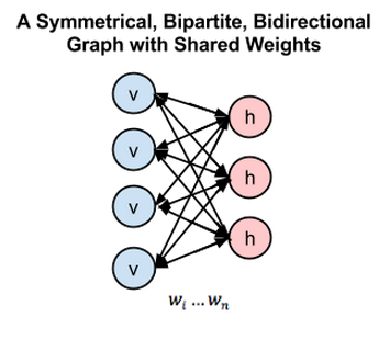
限制玻尔兹曼机并不是一个分类器或者预测模型，而是一个类似于PCA的特征提取模型，它通过一种双层网络来提取数据特征，而这些数据特征可以重构出原来的数据。常用来提取图像和语音特征，结构图如下：

提取结果如下：

2、基本原理：
由于RBM详细原理涉及太多的数学推导，同时还存在物理和数学的交叉理论，其中的许多道理也并不是公式能够说通的，就像爱因斯坦的质能方程一样，它的提出并没有什么道理，无规律可寻，但是它却实实在在的反映了质量和能量的关系，所以这个公式就是有意义的。同样这里的能量和概率的关系也是这样，通过将物理学的能量引入到神经网络，而通过数学推导，其中的能量解释恰好和sigmoid函数相同，因而就能直接通过这种网络来提取特征。

为了直接讲清RBM的原理，这里，我直接说下我的理解，可能不对但也可能提供一些方面的思路：RBM是一个特征提取网络，比如，我们需要造一台翻译机器，可以将某个三维人体画成二维图像，同时，它也能通过二维图像反向重构三维人体，这个简单的原理类似于编解码模型，但是不同的是，这里的编解码使用的是同一个权重，即往返道路是一条。

为了解决上述的问题，我们假设三维是A1，二维是B1，两个操作分别是编码和解码；起初，我们会让编码器根据A1画一张二维图B2，然后让解码器基于画的二维图B2重构三维图A2，通过对比A1和A2就可以判断当前机器的智能程度。但是这里又有一个问题，这样漫无目的的随机画图，如果没有偶然音素，找到一个好的模型基本上是不可能的，所以，我们需要有一个训练方向，一般情况可以直接使用梯度下降或者上升。

但是另一个问题来了，一个样本的训练怎么能够代表整体？因而为了尽可能的学习整体的体征，要么找到一个好的采样方法，要么尽可能的采样直到找到一个能够反映整体样本。显然，我们需要一个好的采样方法来模拟这个过程。

其中Vb\Wn\Hb分别代表可见层偏置\权重\隐藏层偏置，我们需要通过不断地马尔科夫转移，找到一个最合理的An\Bn。

2、基本理论

• Bayes定理：
  

• MCMC蒙特卡罗模型：
  蒙特卡罗是一种通过概率求解积分的算法，如果我们不知道某个函数的积分，但是通过对应函数的概率函数就可以近似模拟对应的积分。比如求解圆周率π，我们可以直接随机一个单位为1的正方形，通过判断落在圆中点的个数就能够近似求解圆周率。进一步，我们这里的x、y是均值分布，如果它的分布并不是均匀分布，而是服从f(x)的分布，就需要更具f(x)来求解，如下：
  

  假设计算，如果无法通过数学推导直接求出解析解，一般不可能对区间(a,b)上所有的x值进行枚举，我们可以将h(x)分解为某个函数f(x)和一个定义在(a,b)上的概率密度函数p(x)的乘积，则整个积分可以写成，这样原积分等同于f(x)在p(x)这个分布上的均值。这时，如果我们从分布p(x)上采集大量的样本点，这些样本符合分布p(x)，即有。那么我们就可以通过这些样本来逼近这个均值，这就是蒙特卡罗方法的基本思想。蒙特卡罗方法的核心问题是如何从分布上随机采集样本，一般采用马尔可夫链蒙特卡罗方法（Markov Chain Monte Carlo，MCMC）产生指定分布下的样本。

• 马尔可夫链：
  马尔科夫链即状态转移函数，把画图和重构比作AB两个过程，通过不断地A-B-A-B-A-B-A-B…最后A和B的分布将近似接近现实的分布。

  离散时间上随机变量随时间变化的转移概率仅仅依赖于当前值的序列，MCMC建立的理论基础：如果我们想在某个分布下采样，只需要模拟以其为平稳分布的马尔科夫过程，经过足够多次转移之后，我们的样本分布就会充分接近于该平稳分布，也就意味着我们近似地采集目标分布下的样本。

3、网络结构：

RBM由两层构成，可见层和隐藏层，分别对因原始数据和特征数据。
构建过程：

即：f(x) = w*x+hb
其中hb为隐藏层偏差

重构过程：

即：h(x) = w*x’+vb
其中vb为可见层偏差

4、理论推导

• 能量函数和概率分布：
  这里作者定义了一个能量函数，而分布的概率是通过能量函数来求解，这里的理论其实并不重要，它的作用就是sigmoid函数的作用。

定义某个分布的概率为：

其中 s 是某个量子态， E(s) 为这个状态的能量， P(s) 为这个状态出现的概率。
考虑到某一个单个单元的状态i，有：

或写为：

这里的E如何设定，由于这个知识设计到物理学知识，它的由来是从物理学变换过来的，公式如下：

对于其中一个隐藏权重hi，我们可以将某个神经元 hi 关联的能量分离出来，也就是：

其中 Wi 是和神经元 hi 相连的权重，h’ 是除去 hi 的向量。
为了方便，我们把和 hi 无关的部分记作：

于是得：

推出：

即最后的结果就是用sigmoid函数作用在状态转移结果上，即：

最终的所有的理论就是一个sigmoid函数：玻尔兹曼分布下隐含层神经元激活的条件概率的激活函数。

最后我们得到隐藏层和可见层的编解码结果：


这里的结果在0-1之间。这里将结果解释为分类对错的能力，1代表对，0代表错。训练目标即最大化似然函数：，一般通过对数转化为连加的形式，其等价形式：
将简记为

• 梯度计算：
  梯度上升法：

由于梯度求解的原理正是找到一个完全符合原始分布的样本，但是这个寻找过程很难，所以，目前的基本方式主要采用吉布斯采样和对比散度来进行训练。

吉布斯采样：每次固定其他特征不变，只训练一个特征。
对比散度：暂留，参照：https://blog.csdn.net/xbinworld/article/details/45274289

5、实实践案例：
example1：sklearn数字图像特征提取

from PIL import Image
import numpy as np
import matplotlib.pyplot as plt
from sklearn.neural_network import BernoulliRBMimg0 = np.array(Image.open('zero.png').convert('L'))#标准化数据，只有0和1的值
def normalize_data(data):  # 0.1<=data[i][j]<=0.9data = (data - np.mean(data)) / np.std(data)rows,cols = data.shapefor i in range(rows):for j in range(cols):if (data[i,j] > 0):data[i,j] = 1else:data[i,j] = 0return dataimg0 = normalize_data(img0)rbm = BernoulliRBM(n_components=20, learning_rate=0.06, batch_size=10, n_iter=200, verbose=True, random_state=0)
rbm.fit(img0)
#得到权值矩阵、隐藏层偏置值和显示层的偏置值
weight = rbm.components_
baise = rbm.intercept_hidden_
baise_vis = rbm.intercept_visible_#逆向还原输入的图片
hidden_img = np.dot(img0, weight.T) + baise
reverimg = np.dot(hidden_img, weight) + baise_vis
#print(reverimg.shape)#图片输出显示
ax = plt.subplot(1, 3, 1)
plt.title('original image')
plt.imshow(img0, cmap='gray')
ax = plt.subplot(1, 3, 2)
plt.title('hidden_img')
plt.imshow(hidden_img, cmap='gray')
ax = plt.subplot(1, 3, 3)
plt.title('reverimg')
plt.imshow(reverimg, cmap='gray')
plt.show()

example2：使用rbm特征做回归分类

"""
==============================================================
Restricted Boltzmann Machine features for digit classification
==============================================================For greyscale image data where pixel values can be interpreted as degrees of
blackness on a white background, like handwritten digit recognition, the
Bernoulli Restricted Boltzmann machine model (:class:`BernoulliRBM
<sklearn.neural_network.BernoulliRBM>`) can perform effective non-linear
feature extraction.In order to learn good latent representations from a small dataset, we
artificially generate more labeled data by perturbing the training data with
linear shifts of 1 pixel in each direction.This example shows how to build a classification pipeline with a BernoulliRBM
feature extractor and a :class:`LogisticRegression
<sklearn.linear_model.LogisticRegression>` classifier. The hyperparameters
of the entire model (learning rate, hidden layer size, regularization)
were optimized by grid search, but the search is not reproduced here because
of runtime constraints.Logistic regression on raw pixel values is presented for comparison. The
example shows that the features extracted by the BernoulliRBM help improve the
classification accuracy.
"""from __future__ import print_functionprint(__doc__)# Authors: Yann N. Dauphin, Vlad Niculae, Gabriel Synnaeve
# License: BSDimport numpy as np
import matplotlib.pyplot as pltfrom scipy.ndimage import convolve
from sklearn import linear_model, datasets, metrics
from sklearn.model_selection import train_test_split
from sklearn.neural_network import BernoulliRBM
from sklearn.pipeline import Pipeline
from sklearn.base import clone# #############################################################################
# Setting updef nudge_dataset(X, Y):"""上下左右四个方向做卷积，4+1=5，复制5倍This produces a dataset 5 times bigger than the original one,by moving the 8x8 images in X around by 1px to left, right, down, up"""direction_vectors = [[[0, 1, 0],[0, 0, 0],[0, 0, 0]],[[0, 0, 0],[1, 0, 0],[0, 0, 0]],[[0, 0, 0],[0, 0, 1],[0, 0, 0]],[[0, 0, 0],[0, 0, 0],[0, 1, 0]]]def shift(x, w):return convolve(x.reshape((8, 8)), mode='constant', weights=w).ravel()X = np.concatenate([X] +[np.apply_along_axis(shift, 1, X, vector)for vector in direction_vectors])Y = np.concatenate([Y for _ in range(5)], axis=0)return X, Y# Load Data
digits = datasets.load_digits()
X = np.asarray(digits.data, 'float32')
X, Y = nudge_dataset(X, digits.target)
# 归一化到0-1
X = (X - np.min(X, 0)) / (np.max(X, 0) + 0.0001)  # 0-1 scalingX_train, X_test, Y_train, Y_test = train_test_split(X, Y, test_size=0.2, random_state=0)# Models we will use
logistic = linear_model.LogisticRegression(solver='lbfgs', max_iter=10000,multi_class='multinomial')
rbm = BernoulliRBM(random_state=0, verbose=True)rbm_features_classifier = Pipeline(steps=[('rbm', rbm), ('logistic', logistic)])# #############################################################################
# Training# Hyper-parameters. These were set by cross-validation,
# using a GridSearchCV. Here we are not performing cross-validation to
# save time.
rbm.learning_rate = 0.06
rbm.n_iter = 20
# More components tend to give better prediction performance, but larger
# fitting time
rbm.n_components = 100 # 隐藏层，相当于特征值
logistic.C = 6000 # 正则化系数λ的倒数，通常默认为1，越大正则化越微小，默认为1# 利用管道一次定义训练，多步使用
# Training RBM-Logistic Pipeline
rbm_features_classifier.fit(X_train, Y_train)# Training the Logistic regression classifier directly on the pixel
raw_pixel_classifier = clone(logistic)
raw_pixel_classifier.C = 100.
raw_pixel_classifier.fit(X_train, Y_train)# #############################################################################
# EvaluationY_pred = rbm_features_classifier.predict(X_test)
print("Logistic regression using RBM features:\n%s\n" % (metrics.classification_report(Y_test, Y_pred)))Y_pred = raw_pixel_classifier.predict(X_test)
print("Logistic regression using raw pixel features:\n%s\n" % (metrics.classification_report(Y_test, Y_pred)))# #############################################################################
# Plottingplt.figure(figsize=(4.2, 4))
for i, comp in enumerate(rbm.components_):plt.subplot(10, 10, i + 1)plt.imshow(comp.reshape((8, 8)), cmap=plt.cm.gray_r,interpolation='nearest')plt.xticks(())plt.yticks(())
plt.suptitle('100 components extracted by RBM', fontsize=16)
plt.subplots_adjust(0.08, 0.02, 0.92, 0.85, 0.08, 0.23)plt.show()

example3：rbm的tensorflow实现-数字图像处理特征提取

"""
Restricted Boltzmann Machines (RBM)
author: Ye Hu
2016/12/18
"""
import os
import timeit
import numpy as np
import tensorflow as tf
from PIL import Image
from unit06_rbm.utils import tile_raster_images
from unit06_rbm import input_dataclass RBM(object):"""A Restricted Boltzmann Machines class"""def __init__(self, inpt=None, n_visiable=784, n_hidden=500, W=None,hbias=None, vbias=None):""":param inpt: Tensor, the input tensor [None, n_visiable]:param n_visiable: int, number of visiable units:param n_hidden: int, number of hidden units:param W, hbias, vbias: Tensor, the parameters of RBM (tf.Variable)"""self.n_visiable = n_visiableself.n_hidden = n_hidden# Optionally initialize inputif inpt is None:inpt = tf.placeholder(dtype=tf.float32, shape=[None, self.n_visiable])self.input = inpt# Initialize the parameters if not givenif W is None:bounds = -4.0 * np.sqrt(6.0 / (self.n_visiable + self.n_hidden))W = tf.Variable(tf.random_uniform([self.n_visiable, self.n_hidden], minval=-bounds,maxval=bounds), dtype=tf.float32)if hbias is None:hbias = tf.Variable(tf.zeros([self.n_hidden, ]), dtype=tf.float32)if vbias is None:vbias = tf.Variable(tf.zeros([self.n_visiable, ]), dtype=tf.float32)self.W = Wself.hbias = hbiasself.vbias = vbias# keep track of parameters for training (DBN)self.params = [self.W, self.hbias, self.vbias]def propup(self, v):"""Compute the sigmoid activation for hidden units given visible units"""return tf.nn.sigmoid(tf.matmul(v, self.W) + self.hbias)def propdown(self, h):"""Compute the sigmoid activation for visible units given hidden units"""return tf.nn.sigmoid(tf.matmul(h, tf.transpose(self.W)) + self.vbias)def sample_prob(self, prob):"""Do sampling with the given probability (you can use binomial in Theano)"""return tf.nn.relu(tf.sign(prob - tf.random_uniform(tf.shape(prob))))def sample_h_given_v(self, v0_sample):"""Sampling the hidden units given visiable sample"""h1_mean = self.propup(v0_sample)h1_sample = self.sample_prob(h1_mean)return (h1_mean, h1_sample)def sample_v_given_h(self, h0_sample):"""Sampling the visiable units given hidden sample"""v1_mean = self.propdown(h0_sample)v1_sample = self.sample_prob(v1_mean)return (v1_mean, v1_sample)def gibbs_vhv(self, v0_sample):"""Implement one step of Gibbs sampling from the visiable state"""h1_mean, h1_sample = self.sample_h_given_v(v0_sample)v1_mean, v1_sample = self.sample_v_given_h(h1_sample)return (h1_mean, h1_sample, v1_mean, v1_sample)def gibbs_hvh(self, h0_sample):"""Implement one step of Gibbs sampling from the hidden state"""v1_mean, v1_sample = self.sample_v_given_h(h0_sample)h1_mean, h1_sample = self.sample_h_given_v(v1_sample)return (v1_mean, v1_sample, h1_mean, h1_sample)def free_energy(self, v_sample):"""Compute the free energy"""wx_b = tf.matmul(v_sample, self.W) + self.hbiasvbias_term = tf.matmul(v_sample, tf.expand_dims(self.vbias, axis=1))hidden_term = tf.reduce_sum(tf.log(1.0 + tf.exp(wx_b)), axis=1)return -hidden_term - vbias_termdef get_train_ops(self, learning_rate=0.1, k=1, persistent=None):"""Get the training opts by CD-k:params learning_rate: float:params k: int, the number of Gibbs step (Note k=1 has been shown work surprisingly well):params persistent: Tensor, PCD-k (TO DO:)"""# Compute the positive phaseph_mean, ph_sample = self.sample_h_given_v(self.input)# The old state of the chainif persistent is None:chain_start = ph_sampleelse:chain_start = persistent# Use tf.while_loop to do the CD-kcond = lambda i, nv_mean, nv_sample, nh_mean, nh_sample: i < kbody = lambda i, nv_mean, nv_sample, nh_mean, nh_sample: (i + 1,) + self.gibbs_hvh(nh_sample)i, nv_mean, nv_sample, nh_mean, nh_sample = tf.while_loop(cond, body, loop_vars=[tf.constant(0),tf.zeros(tf.shape(self.input)),tf.zeros(tf.shape(self.input)),tf.zeros(tf.shape(chain_start)),chain_start])"""# Compute the update values for each parameterupdate_W = self.W + learning_rate * (tf.matmul(tf.transpose(self.input), ph_mean) - tf.matmul(tf.transpose(nv_sample), nh_mean)) / tf.to_float(tf.shape(self.input)[0])  # use probabilityupdate_vbias = self.vbias + learning_rate * (tf.reduce_mean(self.input - nv_sample, axis=0))   # use binary valueupdate_hbias = self.hbias + learning_rate * (tf.reduce_mean(ph_mean - nh_mean, axis=0))       # use probability# Assign the parameters new valuesnew_W = tf.assign(self.W, update_W)new_vbias = tf.assign(self.vbias, update_vbias)new_hbias = tf.assign(self.hbias, update_hbias)"""chain_end = tf.stop_gradient(nv_sample)  # do not compute the gradientscost = tf.reduce_mean(self.free_energy(self.input)) - tf.reduce_mean(self.free_energy(chain_end))# Compute the gradientsgparams = tf.gradients(ys=[cost], xs=self.params)new_params = []for gparam, param in zip(gparams, self.params):new_params.append(tf.assign(param, param - gparam * learning_rate))if persistent is not None:new_persistent = [tf.assign(persistent, nh_sample)]else:new_persistent = []return new_params + new_persistent  # use for trainingdef get_reconstruction_cost(self):"""Compute the cross-entropy of the original input and the reconstruction"""activation_h = self.propup(self.input)activation_v = self.propdown(activation_h)# Do this to not get Nanactivation_v_clip = tf.clip_by_value(activation_v, clip_value_min=1e-30, clip_value_max=1.0)reduce_activation_v_clip = tf.clip_by_value(1.0 - activation_v, clip_value_min=1e-30, clip_value_max=1.0)cross_entropy = -tf.reduce_mean(tf.reduce_sum(self.input * (tf.log(activation_v_clip)) +(1.0 - self.input) * (tf.log(reduce_activation_v_clip)), axis=1))return cross_entropydef reconstruct(self, v):"""Reconstruct the original input by RBM"""h = self.propup(v)return self.propdown(h)if __name__ == "__main__":os.environ['CUDA_VISIBLE_DEVICES'] = '-1'# mnist examplesmnist = input_data.read_data_sets("MNIST_data/", one_hot=True)# define inputx = tf.placeholder(tf.float32, shape=[None, 784])# set random_seedtf.set_random_seed(seed=99999)np.random.seed(123)# the rbm modeln_visiable, n_hidden = 784, 500rbm = RBM(x, n_visiable=n_visiable, n_hidden=n_hidden)learning_rate = 0.1batch_size = 20cost = rbm.get_reconstruction_cost()# Create the persistent variablepersistent_chain = tf.Variable(tf.zeros([batch_size, n_hidden]), dtype=tf.float32)train_ops = rbm.get_train_ops(learning_rate=learning_rate, k=15, persistent=persistent_chain)init = tf.global_variables_initializer()output_folder = "rbm_plots"if not os.path.isdir(output_folder):os.makedirs(output_folder)os.chdir(output_folder)training_epochs = 15display_step = 1print("Start training...")with tf.Session() as sess:start_time = timeit.default_timer()sess.run(init)for epoch in range(training_epochs):avg_cost = 0.0batch_num = int(mnist.train.num_examples / batch_size)for i in range(batch_num):x_batch, _ = mnist.train.next_batch(batch_size)# 训练sess.run(train_ops, feed_dict={x: x_batch})# 计算costavg_cost += sess.run(cost, feed_dict={x: x_batch, }) / batch_num# 输出if epoch % display_step == 0:print("Epoch {0} cost: {1}".format(epoch, avg_cost))# Construct image from the weight matriximage = Image.fromarray(tile_raster_images(X=sess.run(tf.transpose(rbm.W)),img_shape=(28, 28),tile_shape=(10, 10),tile_spacing=(1, 1)))image.save("new_filters_at_epoch_{0}.png".format(epoch))end_time = timeit.default_timer()training_time = end_time - start_timeprint("Finished!")print("  The training ran for {0} minutes.".format(training_time / 60, ))# Reconstruct the image by samplingprint("...Sampling from the RBM")# then_chains = 20n_samples = 10number_test_examples = mnist.test.num_examples# Randomly select the 'n_chains' examplestest_indexs = np.random.randint(number_test_examples - n_chains)test_samples = mnist.test.images[test_indexs:test_indexs + n_chains]# Create the persistent variable saving the visiable statepersistent_v_chain = tf.Variable(tf.to_float(test_samples), dtype=tf.float32)# The step of Gibbsstep_every = 1000# Inplement the Gibbscond = lambda i, h_mean, h_sample, v_mean, v_sample: i < step_everybody = lambda i, h_mean, h_sample, v_mean, v_sample: (i + 1,) + rbm.gibbs_vhv(v_sample)i, h_mean, h_sample, v_mean, v_sample = tf.while_loop(cond, body,loop_vars=[tf.constant(0), tf.zeros([n_chains, n_hidden]),tf.zeros([n_chains, n_hidden]),tf.zeros(tf.shape(persistent_v_chain)),persistent_v_chain])# Update the persistent_v_chainnew_persistent_v_chain = tf.assign(persistent_v_chain, v_sample)# Store the image by samplingimage_data = np.zeros((29 * (n_samples + 1) + 1, 29 * (n_chains) - 1),dtype="uint8")# Add the original imagesimage_data[0:28, :] = tile_raster_images(X=test_samples,img_shape=(28, 28),tile_shape=(1, n_chains),tile_spacing=(1, 1))# Initialize the variablesess.run(tf.variables_initializer(var_list=[persistent_v_chain]))# Do successive samplingfor idx in range(1, n_samples + 1):sample = sess.run(v_mean)sess.run(new_persistent_v_chain)print("...plotting sample", idx)image_data[idx * 29:idx * 29 + 28, :] = tile_raster_images(X=sample,img_shape=(28, 28),tile_shape=(1, n_chains),tile_spacing=(1, 1))image = Image.fromarray(image_data)image.save("new_original_and_{0}samples.png".format(n_samples))

原始图：

参考：
https://zhuanlan.zhihu.com/p/22794772
https://mp.weixin.qq.com/s/1Rek6q-M8pmH5SjYjtPkrA
https://deeplearning4j.org/cn/restrictedboltzmannmachine.html
http://scikit-learn.org/stable/modules/generated/sklearn.neural_network.BernoulliRBM.html

文章：
[1] A Practical Guide to Training Restricted Boltzmann Machines - Geo rey Hinton
[2] A fast learning algorithm for deep belief nets