END-TO-END OPTIMIZED IMAGE COMPRESSION
文章目录
- END-TO-END OPTIMIZED IMAGE COMPRESSION
- 单词
- 摘要:
- 1.INTRODUCTION
- 2.CHOICE OF FORWARD, INVERSE, AND PERCEPTUAL TRANSFORMS
- 3.OPTIMIZATION OF NONLINEAR TRANSFORM CODING MODEL
- 3.1 RELATIONSHIP TO VARIATIONAL GENERATIVE IMAGE MODELS
- 4 EXPERIMENTAL RESULTS
- 5 DISCUSSION
- 实践
- Overview
- Define the trainer model
- Train the model
- Compress some MNIST images
- The rate–distortion trade-off
- Use the decoder as a generative model
- 变分自编码器
- 生成网络
- 推理网络
- 重参数化技巧
- 网络架构
单词
image compression 图像压缩
quantizer 量化器
rate–distortion performance率失真性能
a variant of 什么什么的一个变体
construct 构造
entropy 熵
discrete value 离散值
摘要:
We describe an image compression method, consisting of a nonlinear analysis transformation, a uniform quantizer, and a nonlinear synthesis transformation. The transforms are constructed in three successive stages of convolutional linear filters and nonlinear activation functions. Unlike most convolutional neural networks, the joint nonlinearity is chosen to implement a form of local gain control, inspired by those used to model biological neurons. Using a variant of stochastic gradient descent, we jointly optimize the entire model for rate–distortion performance over a database of training images, introducing a continuous proxy for the discontinuous loss function arising from the quantizer. Under certain conditions, the relaxed loss function may be interpreted as the log likelihood of a generative model, as implemented by a variational autoencoder. Unlike these models, however, the compression model must operate at any given point along the rate– distortion curve, as specified by a trade-off parameter. Across an independent set of test images, we find that the optimized method generally exhibits better rate–distortion performance than the standard JPEG and JPEG 2000 compression methods. More importantly, we observe a dramatic improvement in visual quality for all images at all bit rates, which is supported by objective quality estimates using MS-SSIM.
我们描述了一种图像压缩方法,包括非线性分析变换、均匀量化器和非线性合成变换。这些变换是在卷积线性滤波器和非线性激活函数的三个连续阶段中构造的。与大多数卷积神经网络不同,受用于模拟生物神经元的网络的启发,选择联合非线性来实现一种局部增益控制形式。使用随机梯度下降的变体,我们在训练图像数据库上联合优化整个模型的率失真性能,引入量化器产生的不连续损失函数的连续代理。在某些条件下,松弛损失函数可以解释为由变分自动编码器实现的生成模型的对数似然。然而,与这些模型不同的是,压缩模型必须在速率失真曲线上的任何给定点上运行,如权衡参数所指定。在一组独立的测试图像中,我们发现优化方法通常比标准 JPEG 和 JPEG 2000 压缩方法表现出更好的率失真性能。更重要的是,我们观察到所有比特率下所有图像的视觉质量都有显着改善,这得到了使用 MS-SSIM 的客观质量估计的支持
1.INTRODUCTION
Data compression is a fundamental and well-studied problem in engineering, and is commonly formulated with the goal of designing codes for a given discrete data ensemble with minimal entropy (Shannon, 1948).The solution relies heavily on knowledge of the probabilistic structure of the data, and thus the problem is closely related to probabilistic source modeling. However, since all practical codes must have finite entropy, continuous-valued data (such as vectors of image pixel in- tensities) must be quantized to a finite set of discrete values, which introduces error. In this context, known as the lossy compression problem, one must trade off two competing costs: the entropy of the discretized representation (rate) and the error arising from the quantization (distortion).Different compression applications, such as data storage or transmission over limited-capacity channels, demand different rate–distortion trade-offs.
数据压缩是工程中一个基本且经过充分研究的问题,通常以为给定离散数据集合设计具有最小熵的代码为目标而制定(Shannon,1948)。该解决方案在很大程度上依赖于数据概率结构的知识,因此该问题与概率源建模密切相关。**然而,由于所有实际代码都必须具有有限的熵,因此连续值数据(例如图像像素强度的向量)必须量化为一组有限的离散值,这会引入误差。**在这种情况下,称为有损压缩问题,必须权衡两个相互竞争的成本:离散表示的熵(速率)和量化产生的误差(失真)。不同的压缩应用,例如数据存储或通过有限容量通道传输,需要不同的速率-失真权衡
Joint optimization of rate and distortion is difficult.Without further constraints, the general problem of optimal quantization in high-dimensional spaces is intractable (Gersho and Gray, 1992).For this reason, most existing image compression methods operate by linearly transforming the data vector into a suitable continuous-valued representation, quantizing its elements independently, and then encoding the resulting discrete representation using a lossless entropy code (Wintz, 1972; Netravali and Limb,1980).
速率和失真的联合优化很困难。如果没有进一步的约束,高维空间中最优量化的一般问题是棘手的(Gersho 和 Gray,1992)。因此,大多数现有的图像压缩方法通过将数据向量线性变换为合适的连续值表示,独立量化其元素,然后使用无损熵代码对所得离散表示进行编码(Wintz,1972;Netravali 和 Limb, 1980)。
This scheme is called transform coding due to the central role of the transformation.For example, JPEG uses a discrete cosine transform on blocks of pixels, and JPEG 2000 uses a multi-scale orthogonal wavelet decomposition. Typically, the three components of transform coding methods – transform, quantizer, and entropy code – are separately optimized (often through manual parameter adjustment).
由于变换的核心作用,该方案被称为变换编码。例如,JPEG 对像素块使用离散余弦变换,而 JPEG 2000 使用多尺度正交小波分解。通常,变换编码方法的三个组成部分——变换、量化器和熵代码——是分别优化的(通常通过手动参数调整)。
We have developed a framework for end-to-end optimization of an image compression model based on nonlinear transforms (figure 1).Previously, we demonstrated that a model consisting of linear– nonlinear block transformations, optimized for a measure of perceptual distortion, exhibited visually superior performance compared to a model optimized for mean squared error (MSE) (Ball ́e, La- parra, and Simoncelli,2016).Here, we optimize for MSE, but use a more flexible transforms built from cascades of linear convolutions and nonlinearities.Specifically, we use a generalized divisive normalization (GDN) joint nonlinearity that is inspired by models of neurons in biological visual systems, and has proven effective in Gaussianizing image densities (Ball ́e, Laparra, and Simoncelli, 2015).This cascaded transformation is followed by uniform scalar quantization (i.e., each element is rounded to the nearest integer), which effectively implements a parametric form of vector quantization on the original image space.The compressed image is reconstructed from these quantized values using an approximate parametric nonlinear inverse transform.
我们开发了一个基于非线性变换的图像压缩模型端到端优化框架(图 1)。之前,我们证明了由线性-非线性块变换组成的模型,针对感知失真的测量进行了优化,与针对均方误差(MSE)优化的模型(Ball ́e、Laparra 和 Simoncelli, 2016)。在这里,我们针对 MSE 进行优化,但使用由线性卷积和非线性级联构建的更灵活的变换。具体来说,我们使用广义除法归一化(GDN)联合非线性,其灵感来自生物视觉系统中的神经元模型,并已被证明在高斯化图像密度方面有效(Ball ́e、Laparra 和 Simoncelli,2015)。这种级联变换之后是均匀标量量化(即,每个元素都舍入到最接近的整数),这有效地在原始图像空间上实现了矢量量化的参数形式。使用近似参数非线性逆变换从这些量化值重建压缩图像。
For any desired point along the rate–distortion curve, the parameters of both analysis and synthesis transforms are jointly optimized using stochastic gradient descent.To achieve this in the presence of quantization (which produces zero gradients almost everywhere), we use a proxy loss function based on a continuous relaxation of the probability model, replacing the quantization step with additive uniform noise.The relaxed rate–distortion optimization problem bears some resemblance to those used to fit generative image models, and in particular variational autoencoders (Kingma and Welling, 2014; Rezende, Mohamed, and Wierstra, 2014), but differs in the constraints we impose to ensurethat it approximates the discrete problem all along the rate–distortion curve.Finally, rather than reporting differential or discrete entropy estimates, we implement an entropy code and report performance using actual bit rates, thus demonstrating the feasibility of our solution as a complete lossy compression method.
对于速率失真曲线上的任何所需点,使用随机梯度下降联合优化分析和综合变换的参数。为了在存在量化(几乎在任何地方产生零梯度)的情况下实现这一目标,我们使用基于概率模型的连续松弛的代理损失函数,用加性均匀噪声代替量化步骤。松弛率失真优化问题与用于拟合生成图像模型的问题有一些相似之处,特别是变分自动编码器(Kingma 和 Welling,2014 年;Rezende、Mohamed 和 Wierstra,2014 年),但不同之处在于我们为确保它近似于沿着率失真曲线的离散问题。最后,我们不是报告差分或离散熵估计,而是使用实际比特率实现熵代码并报告性能,从而证明了我们的解决方案作为完整有损压缩方法的可行性。
2.CHOICE OF FORWARD, INVERSE, AND PERCEPTUAL TRANSFORMS
正向、反向和感知变换的选择
Most compression methods are based on orthogonal linear transforms, chosen to reduce correlations in the data, and thus to simplify entropy coding.But the joint statistics of linear filter responses exhibit strong higher order dependencies.These may be significantly reduced through the use of joint localnonlinear gain control operations (Schwartz and Simoncelli, 2001; Lyu, 2010; Sinz and Bethge, 2013), inspired by models of visual neurons (Heeger, 1992; Carandini and Heeger, 2012).Cascaded versions of such models have been used to capturemultiple stages of visual transformation (Simoncelli and Heeger, 1998; Mante, Bonin, and Carandini, 2008).Some earlier results suggest that incorporating local normalization in linear block transform coding methods can improve coding performance (Malo et al., 2006), and can improve object recognition performance of cascaded convolutional neural networks (Jarrett et al., 2009).However, the normalization parameters in these cases were not optimized for the task.Here, we make use of a generalized divisive normalization (GDN) transformwith optimized parameters, that we have previously shown to be highly efficient in Gaussianizing the local joint statistics of natural images, much more so than cascades of linear transforms followed by pointwise nonlinearities (Ball ́e, Laparra, and Simoncelli, 2015)
大多数压缩方法都基于正交线性变换,选择这些方法是为了减少数据中的相关性,从而简化熵编码。但是线性滤波器响应的联合统计表现出强烈的高阶依赖性。通过使用联合局部可以显着减少这些依赖性。非线性增益控制操作(Schwartz 和 Simoncelli,2001;Lyu,2010;Sinz 和 Bethge,2013),受到视觉神经元模型的启发(Heeger,1992;Carandini 和 Heeger,2012)。此类模型的级联版本已用于捕获视觉变换的多个阶段(Simoncelli 和 Heeger,1998;Mante、Bonin 和 Carandini,2008)。一些早期结果表明,在线性块变换编码方法中结合局部归一化可以提高编码性能(Malo 等,2006) ,并且可以提高级联卷积神经网络的对象识别性能(Jarrett et al., 2009)。但是,这些情况下的归一化参数并未针对该任务进行优化。在这里,我们利用广义除法归一化(GDN)变换使用优化的参数,我们之前已经证明它在对自然图像的局部联合统计进行高斯化方面非常有效,比线性变换级联和逐点非线性要高效得多(Ball ́e、Laparra 和 Simoncelli,2015)
Note that some training algorithms for deep convolutional networks incorporate “batch normalization”, rescaling the responses of linear filters in the network so as to keep it in a reasonable operating range (Ioffe and Szegedy, 2015).This type of normalization is different from local gain control in that the rescaling factor is identical across all spatial locations.Moreover, once the training is completed, the scaling parameters are typically fixed, which turns the normalization into an affine transformation with respect to the data – unlike GDN, which is spatially adaptive and can be highly nonlinear.
请注意,深度卷积网络的一些训练算法包含“批量归一化”,重新调整网络中线性滤波器的响应,以使其保持在合理的操作范围内(Ioffe 和 Szegedy,2015)。这种类型的归一化与局部增益控制不同,因为重新缩放因子在所有空间位置上都是相同的。此外,一旦训练完成,缩放参数通常是固定的,这会将归一化转变为针对数据的仿射变换——与空间自适应且高度非线性的 GDN 不同。
Specifically, our analysis transform ga consists of three stages of convolution, subsampling, and divisive normalization.We represent the ith input channel of the kth stage at spatial location (m, n) as u(k) i (m, n).The input image vector x corresponds to u(0) i (m, n), and the output vector y is u(3) i (m, n).Each stage then begins with an affine convolution:
具体来说,我们的分析变换 g a g_a ga 由卷积、子采样和除法归一化三个阶段组成。我们将空间位置 (m, n) 处第 k 级的第 i 个输入通道表示为$ u^{(k)} i (m, n) 。输入图像向量 x 对应于 。输入图像向量x对应于 。输入图像向量x对应于u^{(0)} i (m, n) ,输出向量 y 为 ,输出向量y为 ,输出向量y为u^{(3)}_ i (m, n)$。然后每个阶段都从仿射卷积开始:
(1)
where ∗ denotes 2D convolution. This is followed by downsampling:
其中*表示2D卷积。接下来是下采样:
(2)
where sk is the downsampling factor for stage k.Each stage concludes with a GDN operation
其中 s k s_k sk 是阶段 k 的下采样因子。每个阶段都以 GDN 操作结束
(3)
The full set of h, c, β, and γ parameters (across all three stages) constitute the parameter vector φ to be optimized
全套 h、c、β 和 γ 参数(跨所有三个阶段)构成要优化的参数向量 φ
Analogously, the synthesis transform gs consists of three stages, with the order of operations re- versed within each stage, downsampling replaced by upsampling, and GDN replaced by an approx- imate inverse we call IGDN (more details in the appendix).We define ˆu(k) i (m, n) as the input to the kth synthesis stage, such that ˆy corresponds to ˆu(0) i (m, n), and ˆx to ˆu(3) i (m, n).Each stage then consists of the IGDN operation:
类似地,合成变换 $g_s 由三个阶段组成,每个阶段内的操作顺序颠倒,下采样被上采样取代, G D N 被我们称为 I G D N 的近似逆代替(更多详细信息参见附录)。我们将 由三个阶段组成,每个阶段内的操作顺序颠倒,下采样被上采样取代,GDN 被我们称为 IGDN 的近似逆代替(更多详细信息参见附录)。我们将 由三个阶段组成,每个阶段内的操作顺序颠倒,下采样被上采样取代,GDN被我们称为IGDN的近似逆代替(更多详细信息参见附录)。我们将 \hat{u}^{(k)}_ i (m, n) $定义为第 k 个合成阶段的输入,使得 $\hat y $对应于 u ^ i ( 0 ) ( m , n ) \hat u^{(0)}_ i (m, n) u^i(0)(m,n),而 x ^ \hat x x^ 对应于$ \hat u^{(3)}_ i (m, n)$ 。每个阶段都包含 IGDN 操作:
(4)
which is followed by upsampling
接下来是上采样
(5)
where ˆsk is the upsampling factor for stage k.Finally, this is followed by an affine convolution:
其中 $\hat s_k $是阶段 k 的上采样因子。最后,进行仿射卷积:
(6)
Analogously, the set of ˆh, ˆc, ˆβ, and ˆγ make up the parameter vector θ.Note that the down- /upsampling operations can be implemented jointly with their adjacent convolution, improving com- putational efficiency.
类似地, h ^ \hat h h^、 c ^ \hat c c^、 β ^ \hat β β^ 和$ \hat γ$ 的集合构成了参数向量 θ。请注意,下采样/上采样操作可以与其相邻卷积联合实现,从而提高计算效率。
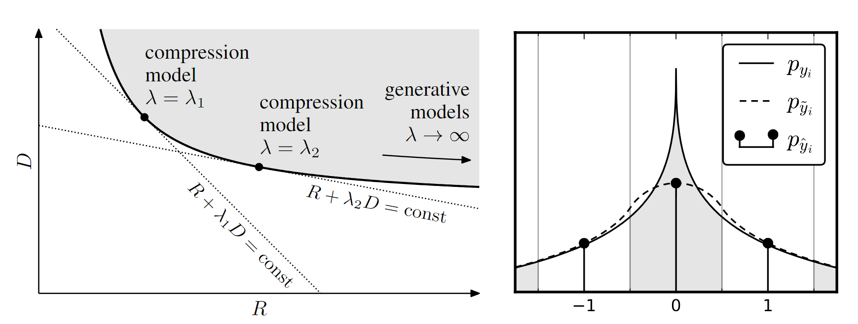
Figure 2:Left: The rate–distortion trade-off.The gray region represents the set of all rate–distortion values that can be achieved (over all possible parameter settings).Optimal performance for a given choice of λ corresponds to a point on the convex hullof this set with slope −1/λ.Right: One- dimensional illustration of relationship between densities of yi (elements of code space), ˆyi (quan- tized elements), and ̃yi (elements perturbed by uniform noise).Each discrete probabilityin pˆyi equals the probability mass of the density pyi within the corresponding quantization bin (indicated by shading).The density p ̃yi provides a continuous function that interpolates the discrete probability values pˆyi at integer positions
左:率失真权衡。灰色区域表示可以实现的所有率失真值的集合(在所有可能的参数设置上)。给定 λ 选择的最佳性能对应于凸包上的点该集合的斜率为−1/λ。右图: y i y_i yi(代码空间元素)、 y ^ i \hat y_i y^i(量化元素)和 y ~ i \widetilde y_i y i(受均匀噪声扰动的元素)密度之间关系的一维图示。每个离散概率$ p_{\hat yi} $等于相应量化仓内密度 $p_{yi} 的概率质量(由阴影表示)。密度 p ~ y i 提供了一个连续函数,可在整数位置插值离散概率值 的概率质量(由阴影表示)。密度 p̃yi 提供了一个连续函数,可在整数位置插值离散概率值 的概率质量(由阴影表示)。密度p~yi提供了一个连续函数,可在整数位置插值离散概率值 p_{ \hat y_i}$
In previous work, we used a perceptual transform gp, separately optimized to mimic human judgements of grayscale image distortions (Laparra et al., 2016), and showed that a set of one-stage transforms optimized for this distortion measure ledto visually improved results (Ball ́e, Laparra, and Simoncelli, 2016).Here, we set the perceptual transform gp to the identity, and use mean squared error (MSE) as the metric (i.e., d(z, ˆz) = ‖z − ˆz‖2 2).This allows a more interpretable comparison to existing methods, which are generally optimized for MSE, and also allows optimization for color images, for which we do not currently have a reliable perceptual metric.
在之前的工作中,我们使用了感知变换$ g_pKaTeX parse error: Expected 'EOF', got '́' at position 75: …致视觉效果得到改善(Ball ̲́e、Laparra 和 Sim… g_p$ 设置为恒等式,并使用均方误差(MSE)作为度量(即 d(z, ˆz) = ‖z − ˆz‖2 2)。这允许与现有方法进行更可解释的比较,这些方法通常针对 MSE 进行优化,并且还允许对彩色图像进行优化,而我们目前还没有可靠的感知指标。
3.OPTIMIZATION OF NONLINEAR TRANSFORM CODING MODEL
非线性变换编码模型的优化
Our objective is to minimize a weighted sum of the rate and distortion, R + λD, over the parameters of the analysis and synthesis transforms and the entropy code, where λ governs the trade-off between the two terms (figure 2, left panel).Rather than attempting optimal quantization directly in the image space, which is intractable due to the high dimensionality, we instead assume a fixed uniform scalar quantizer in the code space, and aim to have the nonlinear transformations warp the space in an appropriate way, effectively implementinga parametric form of vector quantization (figure 1).The actual rates achieved by a properly designed entropy code are only slightly larger than the entropy (Rissanen and Langdon, 1981), and thus we define the objective functional directly in terms of entropy
我们的目标是在分析和综合变换以及熵代码的参数上最小化速率和失真的加权和 R + λD,其中 λ 控制两项之间的权衡(图 2,左图) 。我们不是直接在图像空间中尝试最佳量化(由于高维度而难以处理),而是在代码空间中假设一个固定的均匀标量量化器,并旨在让非线性变换以适当的方式扭曲空间,从而有效地实现矢量量化的参数形式(图 1)。正确设计的熵代码实现的实际速率仅略大于熵(Rissanen 和 Langdon,1981),因此我们直接根据熵定义目标函数
(7)
where both expectations will be approximated by averages over a training set of images.Given a powerful enough set of transformations, we can assume without loss of generality that the quantization bin size is always one and the representing values are at the centers of the bins.That is
其中两个期望将通过训练图像集的平均值来近似。给定一组足够强大的变换,我们可以不失一般性地假设量化箱大小始终为 1 并且表示值位于箱的中心。那是
(8)
where index i runs over all elements of the vectors, including channels and spatial locations.The marginal density of ˆyi is then given by a train of discrete probability masses (Dirac delta functions, figure 2, right panel) with weights equal to the probability mass function of qi
其中索引 i 遍历向量的所有元素,包括通道和空间位置。然后,^yi 的边际密度由一系列离散概率质量(狄拉克 δ 函数,图 2,右图)给出,其权重等于 qi 的概率质量函数
(9)
Note that both terms in (7) depend on the quantized values, and the derivatives of the quantization
function (8) are zero almost everywhere, rendering gradient descent ineffective. To allow optimization via stochastic gradient descent, we replace the quantizer with an additive i.i.d. uniform noise source ∆y, which has the same width as the quantization bins (one). This relaxed formulation has two desirable properties. First, the density function of ̃y = y + ∆y is a continuous relaxation of the probability mass function of q (figure 2, right panel):
请注意,公式(7)中的两个项都依赖于量化值,并且量化函数(公式(8))的导数几乎处处为零,使得梯度下降方法无效。为了能够通过随机梯度下降进行优化,我们将量化器替换为一个具有与量化区间(为一)相同宽度的加性独立同分布均匀噪声源∆y。这种松弛的表述具有两个可取之处。首先, y ~ \widetilde y y = y + ∆y的密度函数是q的概率质量函数的连续松弛(见图2的右图)。
(10)
which implies that the differential entropy of ̃y can be used as an approximation of the entropy of q.Second, independent uniform noise approximates quantization error in terms of its marginal moments, and is frequently used as a model of quantization error (Gray and Neuhoff,1998).We can thus use the same approximation for our measure of distortion.We examine the empirical quality of these rate and distortion approximations in section 4
这意味着 ̃y 的微分熵可以用作 q 熵的近似值。 其次,独立均匀噪声根据其边缘矩来近似量化误差,并且经常用作量化误差的模型(Gray 和 Neuhoff, 1998)。因此,我们可以使用相同的近似值来衡量失真。我们在第 4 节中检查了这些速率和失真近似值的经验质量
We assume independent marginals in the code space for both the relaxed probability model of ̃y and the entropy code, and model the marginals p ̃yi non-parametrically to reduce model error.Specifically, we use finely sampled piecewise linear functions which we update similarly to one- dimensional histograms (see appendix).Since p ̃yi = pyi ∗ U(0, 1) is effectively smoothed by a box-car filter – the uniform density on the unit interval, U(0, 1) – the model error can be made arbitrarily small by decreasing the sampling interval
我们假设 ̃y 的宽松概率模型和熵代码在代码空间中具有独立的边际,并对边际 p ̃yi 非参数建模以减少模型误差。具体来说,我们使用精细采样的分段线性函数,其更新方式与一维直方图类似(参见附录)。由于 p ̃yi = pyi ∗ U(0, 1) 通过箱车滤波器有效平滑——单位间隔 U(0, 1) 上的均匀密度——通过减小采样间隔可以使模型误差任意小
Given this continuous approximation of the quantized coefficient distribution, the loss function for
parameters θ and φ can be written as:
给定量化系数分布的连续近似,参数 θ 和 φ 的损失函数可以写为:
(11)
where vector ψ(i) parameterizes the piecewise linear approximation of p ̃yi (trained jointly with θ and φ).This is continuous and differentiable, and thus well-suited for stochastic optimization.
其中向量 ψ(i) 参数化 p ̃yi 的分段线性近似(与 θ 和 φ 联合训练)。这是连续且可微的,因此非常适合随机优化。

Figure 3: Representation of the relaxed rate–distortion optimization problem as the encoder and decoder graphs of a variational autoencoder.Nodes represent random variables, and gray shading indicates observed data;small filled nodes represent parameters;arrows indicate dependency;and nodes within boxes are per-image
图 3:将松弛率失真优化问题表示为变分自编码器的编码器和解码器图。节点代表随机变量,灰色阴影表示观测数据;小的填充节点代表参数;箭头表示依赖关系;框内的节点是针对每个图像的
3.1 RELATIONSHIP TO VARIATIONAL GENERATIVE IMAGE MODELS
与变分生成图像模型的关系
We derived our formulation directly from the classical rate–distortion optimization problem.How- ever, once the transition to a continuous loss function is made, the optimization problem resembles those encountered in fitting generative models of images, and can more specifically be cast in the context of variational autoencoders (Kingma and Welling, 2014; Rezende, Mohamed, and Wierstra, 2014).In Bayesian variational inference, we are given an ensemble of observations of a random variable x along with a generative model px|y (x|y).We seek to find a posterior py|x(y|x), which generally cannot be expressed in closed form.The approach followed by Kingma and Welling (2014) consists of approximating this posterior with a density q(y|x), by minimizing the Kullback– Leibler divergence between the two
我们直接从经典的率失真优化问题中得出公式。然而,一旦过渡到连续损失函数,优化问题类似于拟合图像生成模型时遇到的问题,并且可以更具体地在变分自动编码器的背景下进行转换(Kingma 和 Welling,2014;Rezende,Mohamed) ,和 Wierstra,2014)。在贝叶斯变分推理中,我们得到随机变量 x 的观测值集合以及生成模型 px|y (x|y)。我们寻求找到后验 py|x(y|x),它通常不能以封闭形式表示。 Kingma 和 Welling (2014) 采用的方法包括通过最小化两者之间的 Kullback-Leibler 散度,用密度 q(y|x) 来近似该后验
(12)
This objective function is equivalent to our relaxed rate–distortion optimization problem, with dis- tortion measured as MSE, if we define the generative model as follows (figure 3):
如果我们按如下方式定义生成模型(图 3),则该目标函数相当于我们的宽松率失真优化问题,其中失真测量为 MSE:
(13)
(14)
and the approximate posterior as follows:
以及近似后验如下:
(15)
where U( ̃yi; yi, 1) is the uniform density on the unit interval centered on yi.With this, the first term in the Kullback–Leibler divergence is constant;the second term corresponds to the distortion, and the third term corresponds to the rate (both up to additive constants).Note that if a perceptual transform gp is used, or the metric d is not Euclidean, px|̃y is no longer Gaussian, and equivalence to variational autoencoders cannot be guaranteed, since the distortion term may not correspond to a normalizable density.For any affine and invertible perceptual transform and any translation-invariant metric, it can be shown to correspond to the density
其中U(̃yi;yi,1)是以yi为中心的单位区间上的均匀密度。这样,Kullback-Leibler 散度中的第一项是恒定的;第二项对应于失真,第三项对应于速率(两者都达到加性常数)。请注意,如果使用感知变换 gp,或者度量 d 不是欧几里德,则 px| ̃y 不再是高斯分布,并且不能保证与变分自动编码器的等价性,因为失真项可能不对应于可归一化的密度。对于任何仿射和可逆感知变换以及任何平移不变度量,它可以被证明对应于密度
(16)
其中 Z(λ) 对密度进行归一化(但无需计算以拟合模型)。
Despite the similarity between our nonlinear transform coding framework and that of variational autoencoders, it is worth noting several fundamental differences.First, variational autoencoders are continuous-valued, and digital compression operates in the discrete domain.Comparing differential entropy with (discrete) entropy, or entropy with an actual bit rate, can potentially lead to misleading results.In this paper, we use the continous domain strictly for optimization, and perform the evalu- ation on actual bit rates, which allows comparison to existing image coding methods.We assess the quality of the rate and distortion approximations empirically.
尽管我们的非线性变换编码框架与变分自动编码器之间有相似之处,但值得注意的是几个基本差异。首先,变分自动编码器是连续值的,并且数字压缩在离散域中操作。将微分熵与(离散)熵或熵与实际比特率进行比较可能会导致误导结果。在本文中,我们严格使用连续域进行优化,并对实际比特率进行评估,这可以与现有的图像编码方法进行比较。我们根据经验评估速率和失真近似的质量。
Second, generative models aim to minimize differential entropy of the data ensemble under the model, i.e., explaining fluctuations in the data.This often means minimizing the variance of a “slack” term like (13), which in turn maximizes λ.Transform coding methods, on the other hand, are optimized to achieve the best trade-off between having the model explain the data (which in- creases rate and decreases distortion), and having the slack term explain the data (which decreases rate and increasesdistortion).The overall performance of a compression model is determined by the shape of the convex hull of attainable model distortions and rates, over all possible values of the model parameters.Finding this convex hull is equivalent to optimizing the model for particular values of λ (see figure 2).In contrast, generative models operate in a regime where λ is inferred and ideally approaches infinity for noiseless data, which corresponds to the regime of lossless compres- sion.Even so, lossless compression methods still need to operate in a discretized space, typically directly on quantized luminance values.For generative models, the discretization of luminance val- ues is usually considered a nuisance (Theis, van den Oord, and Bethge, 2015), although there are examples of generative models that operate on quantized pixel values (van den Oord, Kalchbrenner, andKavukcuoglu, 2016)
其次,生成模型旨在最小化模型下数据集合的微分熵,即解释数据的波动。这通常意味着最小化“松弛”项(如(13))的方差,从而最大化 λ。另一方面,变换编码方法经过优化,可以在模型解释数据(增加速率并减少失真)和松弛项解释数据(降低速率并增加失真)之间实现最佳权衡。失真)。压缩模型的整体性能由模型参数的所有可能值上可达到的模型畸变和率的凸包形状决定。找到这个凸包相当于针对特定的 λ 值优化模型(见图 2)。相比之下,生成模型在 λ 被推断的情况下运行,对于无噪声数据理想地接近无穷大,这对应于无损压缩的情况。即便如此,无损压缩方法仍然需要在离散空间中操作,通常直接在量化的亮度值上操作。对于生成模型,亮度值的离散化通常被认为是一件麻烦事(Theis、van den Oord 和 Bethge,2015),尽管有一些生成模型对量化像素值进行操作的示例(van den Oord、Kalchbrenner 和卡武克措格鲁,2016)
Finally, although correspondence between the typical slack term (13) of a generative model (figure 3, left panel) and the distortion metric in rate–distortion optimization holds for simple metrics (e.g., Euclidean distance), a more general perceptual measure would beconsidered a peculiar choice from a generative modeling perspective, if it corresponds to a density at all
最后,虽然生成模型的典型松弛项 (13)(图 3,左图)与率失真优化中的失真度量之间的对应关系对于简单度量(例如欧几里德距离)而言成立,但更一般的感知度量将是如果它完全对应于密度,那么从生成建模的角度来看,它被认为是一个特殊的选择
4 EXPERIMENTAL RESULTS
We jointly optimized the full set of parameters φ, θ, and all ψ over a subset of the ImageNet database (Deng et al., 2009) consisting of 6507 images using stochastic descent.This optimization was performed separately for each λ, yielding separate transforms and marginal probability models for each value.
我们使用随机下降法联合优化了由 6507 张图像组成的 ImageNet 数据库子集(Deng 等人,2009 年)的全套参数 φ、θ 和所有 ψ。这种优化是针对每个 λ 单独执行的,为每个值生成单独的变换和边际概率模型。
For the grayscale analysis transform, we used 128 filters (size 9 × 9) in the first stage, each sub- sampled by a factor of 4 vertically and horizontally.The remaining two stages retain the number of channels, but use filters operating across all input channels (5 × 5 × 128), with outputs subsampled by a factor of 2 in each dimension.The net output thus has half the dimensionality of the input.The synthesis transform is structured analogously.For RGB images, we trained a separate set of models, with the first stage augmented to operate across three (color) input channels.For the two largest values of λ, and for RGB models, we increased the network capacity by increasing the number of channels in each stage to 256 and 192, respectively.Further details about the parameterization of the transforms and their training can be found in the appendix
对于灰度分析变换,我们在第一阶段使用 128 个滤波器(大小 9 × 9),每个滤波器在垂直和水平方向上进行 4 倍的子采样。其余两个阶段保留通道数,但使用在所有输入通道 (5 × 5 × 128) 上运行的滤波器,输出在每个维度上按 2 倍子采样。因此,净输出的维数是输入的一半。合成变换的结构类似。对于 RGB 图像,我们训练了一组单独的模型,第一阶段经过增强,可以跨三个(颜色)输入通道进行操作。对于 λ 的两个最大值和 RGB 模型,我们通过将每个阶段的通道数分别增加到 256 和 192 来增加网络容量。有关变换参数化及其训练的更多详细信息,请参阅附录
We first verified that the continuously-relaxed loss function given in section 3 provides a good ap- proximation to the actual rate–distortion values obtained with quantization (figure 4).The relaxed distortion term appears to be mostly unbiased, and exhibits a relatively small variance.The relaxed (differential) entropy provides a somewhat positively biased estimate of the discrete entropy for the coarser quantization regime, but the bias disappears for finer quantization, as expected.Note that since the values of λ do not have any intrinsic meaning, but serve only to map out the convex hull of optimal points in the rate–distortion plane (figure 2, left panel), a constant bias in either of the terms would simplyalter the effective value of λ, with no effect on the compression performance
我们首先验证了第 3 节中给出的连续松弛损失函数可以很好地逼近通过量化获得的实际率失真值(图 4)。松弛失真项看起来大部分是无偏的,并且表现出相对较小的方差。松弛(微分)熵为较粗的量化机制提供了离散熵的某种正偏差估计,但正如预期的那样,对于更精细的量化,偏差消失了。请注意,由于 λ 的值没有任何内在含义,而仅用于绘制率失真平面中最优点的凸包(图 2,左图),因此任何一项中的恒定偏差都将简单地表示为改变λ的有效值,不影响压缩性能
We compare the rate–distortion performance of our method to two standard methods: JPEG and JPEG 2000. For our method, all images were compressed using uniform quantization (the contin- uous relaxation using additive noise was used only for training purposes).To make the compar- isons more fair, we implemented a simple entropy code based on the context-based adaptive binary arithmetic coding framework (CABAC; Marpe, Schwarz, and Wiegand, 2003).All sideband in- formation needed by the decoder (size of images, value of λ, etc.) was included in the bit stream (see appendix).Note that although the computational costs for training our models are quite high, encoding or decoding an image with the trained models is efficient, requiring only execution of the optimized analysis transformation and quantizer, or the synthesis transformation, respectively.Evaluations were performed on the Kodak image dataset1, an uncompressed set of images com- monly used to evaluate image compression methods.We also examined a set of relatively standard (if outdated) images used by the compression community (known by the names “Lena”, “Barbara”, “Peppers”, and “Mandrill”) as well as a set of our own digital photographs.None of these test images was included in the training set.All test images, compressed at a variety of bit rates us- ing all three methods, along with their associated rate–distortion curves, are available online at http://www.cns.nyu.edu/ ̃lcv/iclr2017
我们将我们的方法与两种标准方法的率失真性能进行比较:JPEG 和 JPEG 2000。对于我们的方法,所有图像都使用均匀量化进行压缩(使用加性噪声的连续松弛仅用于训练目的)。为了使比较更加公平,我们基于基于上下文的自适应二进制算术编码框架(CABAC;Marpe、Schwarz 和 Wiegand,2003)实现了一个简单的熵代码。解码器所需的所有边带信息(图像大小、λ 值等)都包含在比特流中(参见附录)。请注意,尽管训练模型的计算成本相当高,但使用训练模型对图像进行编码或解码是高效的,只需要分别执行优化的分析变换和量化器或合成变换。评估是在柯达图像数据集1上进行的,这是一组未压缩的图像,通常用于评估图像压缩方法。我们还检查了压缩社区使用的一组相对标准(如果过时)的图像(名称为“Lena”、“Barbara”、“Peppers”和“Mandrill”)以及一组我们自己的数码照片。这些测试图像均未包含在训练集中。使用所有三种方法以各种比特率压缩的所有测试图像及其相关的率失真曲线均可在线获取:http://www.cns.nyu.edu/̃lcv/iclr2017
Although we used MSE as a distortion metric for training, the appearance of compressed images is both qualitatively different and substantially improved, compared to JPEG and JPEG 2000. As an example, figure 5 shows an image compressed using our method optimized for a low value ofλ(and thus, a low bit rate), compared to JPEG/JPEG 2000 images compressed at equal or greater bit rates.The image compressed with our method has less detail than the original (not shown, but available online), with fine texture andother patterns often eliminated altogether, but this is accomplished in a way that preserves the smoothness of contours and sharpness of many of theedges, giving them a natural appearance.By comparison, the JPEG and JPEG 2000 images exhibit artifacts that are com- mon to alllinear transform coding methods: since local features (edges, contours, texture elements, etc.) are represented using particularcombinations of localized linear basis functions, independent scalar quantization of the transform coefficients causes imbalances in these combinations, and leads to visually disturbing blocking, aliasing, and ringing artifacts that reflect the underlying basis func- tions
尽管我们使用 MSE 作为训练的失真度量,但与 JPEG 和 JPEG 2000 相比,压缩图像的外观在质量上有所不同,并且得到了显着改善。作为示例,图 5 显示了使用我们针对低 λ 值进行优化的方法压缩的图像(因此,比特率较低),与以相同或更高比特率压缩的 JPEG/JPEG 2000 图像相比。使用我们的方法压缩的图像的细节少于原始图像(未显示,但可在线获取),具有精细的纹理和其他图案通常会被完全消除,但这是通过保留轮廓的平滑度和许多边缘的清晰度来实现的,从而使它们具有自然的外观。相比之下,JPEG 和 JPEG 2000 图像表现出所有图像都常见的伪影。线性变换编码方法:由于局部特征(边缘、轮廓、纹理元素等)是使用局部线性基函数的特定组合来表示的,因此变换系数的独立标量量化会导致这些组合中的不平衡,并导致视觉上令人不安的块、混叠,以及反映底层基函数的振铃伪影
Remarkably, we find that the perceptual advantages of our method hold for all images tested, and at all bit rates.The progression from high to low bit rates is shown for an example image in figure 6 (additional examples provided in appendix and online).As bit rate is reduced, JPEG and JPEG 2000 degrade their approximation of the original image by coarsening the precision of the coefficients of linear basis functions, thus exposing the visual appearance of those basis functions.On the other hand, our method appears to progressively simplify contours and other image features, effectively concealing the underlying quantization of the representation.Consistent with the appearance of these example images, we find that distortion measured with a perceptual metric (MS-SSIM; Wang, Simoncelli, and Bovik, 2003), indicates substantial improvements across all tested images and bit rates (figure 7; additional examples providedin the appendix and online).Finally, when quantified with PSNR, we find that our method exhibits better rate–distortion performance than both JPEG and JPEG 2000 for most (but not all) test images, especially at the lower bit rates
值得注意的是,我们发现我们的方法的感知优势适用于所有测试的图像和所有比特率。图 6 中的示例图像显示了从高比特率到低比特率的进展(附录和在线提供了其他示例)。随着比特率的降低,JPEG 和 JPEG 2000 通过粗化线性基函数系数的精度来降低原始图像的近似值,从而暴露这些基函数的视觉外观。另一方面,我们的方法似乎逐渐简化轮廓和其他图像特征,有效隐藏了表示的底层量化。与这些示例图像的外观一致,我们发现使用感知度量(MS-SSIM;Wang、Simoncelli 和 Bovik,2003)测量的失真表明所有测试图像和比特率都有显着改善(图 7;提供了其他示例)见附录和在线)。最后,当使用 PSNR 进行量化时,我们发现对于大多数(但不是全部)测试图像,我们的方法比 JPEG 和 JPEG 2000 表现出更好的率失真性能,尤其是在较低比特率下
5 DISCUSSION
We have presented a complete image compression method based on nonlinear transform coding, and a framework to optimize it end-to-end for rate–distortion performance.Our compression method of- fers improvements in rate–distortion performance over JPEG and JPEG 2000 for most images and bit rates.More remarkably, although the method was optimized using mean squared error as a dis- tortion metric, the compressed images are much more natural in appearance than those compressed with JPEG or JPEG 2000, both of which suffer from the severe artifacts commonly seen in linear transformcoding methods.Consistent with this, perceptual quality (as estimated with the MS-SSIM index) exhibits substantial improvement across all test images and bit rates.We believe this visual improvement arises because the cascade of biologically-inspired nonlinear transformations in the model have been optimized to capture the features and attributes of images that are represented in the statistics of the data, parallel to the processes of evolution and development that are believedto have shaped visual representations within the human brain (Simoncelli and Olshausen, 2001).Nevertheless, additional visual improvements might be possible if the method were optimized using a perceptual metric in place of MSE (Ball ́e, Laparra, and Simoncelli, 2016)
我们提出了一种基于非线性变换编码的完整图像压缩方法,以及一个端到端优化其率失真性能的框架。对于大多数图像和比特率,我们的压缩方法比 JPEG 和 JPEG 2000 提供了率失真性能的改进。更值得注意的是,尽管该方法使用均方误差作为失真度量进行了优化,但压缩后的图像在外观上比使用 JPEG 或 JPEG 2000 压缩的图像要自然得多,后两者都存在线性变换中常见的严重伪影。编码方法。与此一致的是,感知质量(根据 MS-SSIM 指数估计)在所有测试图像和比特率上都表现出显着改善。我们相信这种视觉改进的出现是因为模型中受生物学启发的非线性变换的级联已经过优化,以捕获数据统计中表示的图像的特征和属性,与人们认为的进化和发展过程平行在人脑中形成视觉表征(Simoncelli 和 Olshausen,2001)。尽管如此,如果使用感知指标代替 MSE 来优化该方法,则可能会获得额外的视觉改进(Ball ́e、Laparra 和 Simoncelli,2016)
For comparison to linear transform coding methods, we can interpret our analysis transform as a single-stage linear transform followed by a complex vector quantizer.As in many other optimized representations – e.g., sparse coding (Lewicki and Olshausen, 1998) – as well as many engineered representations – e.g., the steerable pyramid (Simoncelli, Freeman, et al., 1992), curvelets (Cand`es and Donoho, 2002), and dual-tree complex wavelets (Selesnick, Baraniuk, and Kingsbury, 2005) – the filters in this first stage are localized and oriented and the representation is overcomplete.Whereas most transform coding methods use complete (often orthogonal) linear transforms with spatially separable filters, the overcompleteness and orientation tuning of our initial transform may explain the ability of the model to better represent features and contours with continuously varying orientation, position and scale (Simoncelli, Freeman, et al., 1992).
为了与线性变换编码方法进行比较,我们可以将我们的分析变换解释为单级线性变换,然后是复矢量量化器。与许多其他优化表示一样 - 例如,稀疏编码(Lewicki 和 Olshausen,1998) - 以及许多工程表示 - 例如,可操纵金字塔(Simoncelli,Freeman 等人,1992),曲线(Cand`es 和 Donoho) ,2002)和双树复小波(Selesnick、Baraniuk 和 Kingsbury,2005)——第一阶段的滤波器是局部化和定向的,并且表示是过度完整的。虽然大多数变换编码方法使用具有空间可分离滤波器的完整(通常是正交)线性变换,但我们初始变换的过度完整性和方向调整可以解释模型更好地表示具有连续变化的方向、位置和尺度的特征和轮廓的能力(Simoncelli ,弗里曼等人,1992)。
Our work is related to two previous publications that optimize image representations with the goal of image compression.Gregor, Besse, et al.(2016) introduce an interesting hierarchical representa- tion of images, in which degradations are more natural looking than those of linear representations.However, rather than optimizing directly for rate–distortion performance, their modeling is genera- tive.Due to the differences between these approaches (as outlined in section 3.1), their procedure of obtaining coding representations from the generative model (scalar quantization, and elimination of hierarchical levels of the representation) is less systematic than our approach and unlikely to be optimal.Further, no entropy code is provided, and the authors therefore resort to comparing entropy estimates to bit rates of established compression methods, which can be unreliable.The model developed by Toderici et al.(2016) is optimized to provide various rate–distortion trade-offs and directly output a binary representation, making it more easily comparable to other image compres- sion methods.Moreover, their formulation has the advantage over ours that a single representation is sought for all rate points.However, it is not clear whether their formulation necessarily leads to rate–distortion optimality (and their empirical results suggest that this is not the case).
我们的工作与之前的两篇出版物相关,它们以图像压缩为目标优化图像表示。格雷戈尔、贝斯等人。 (2016)引入了一种有趣的图像分层表示,其中降级比线性表示看起来更自然。然而,他们的建模是生成式的,而不是直接优化率失真性能。由于这些方法之间的差异(如第 3.1 节所述),它们从生成模型获取编码表示的过程(标量量化和消除表示的层次级别)不如我们的方法系统化,并且不太可能是最优的。此外,没有提供熵代码,因此作者将熵估计与已建立的压缩方法的比特率进行比较,这可能是不可靠的。该模型由 Toderici 等人开发。 (2016)经过优化,提供各种率失真权衡并直接输出二进制表示,使其更容易与其他图像压缩方法进行比较。此外,他们的公式比我们的公式具有优势,即为所有费率点寻求单一表示。然而,尚不清楚他们的表述是否必然导致率失真最优(他们的经验结果表明情况并非如此)。
We are currently testing models that use simpler rectified-linear or sigmoidal nonlinearities, to de- termine how much of the performance and visual quality of our results is due to use of biologically- inspired joint nonlinearities.Preliminary results indicate that qualitatively similar results are achiev- able with other activation functions we tested, but that rectified linear units generally require a sub- stantially larger number of model parameters/stages to achieve the same rate–distortion performance as the GDN/IGDN nonlinearities.This suggests that GDN/IGDN transforms are more efficient for compression, producing better models with fewer stages of processing (as we previously found for density estimation; Ball ́e, Laparra, and Simoncelli, 2015), which might be an advantage for de- ploymentof our method, say, in embedded systems.However, such conclusions are based on a somewhat limited set of experiments and should at this point be considered provisional.More gen- erally, GDN represents a multivariate generalization of a particular type of sigmoidal function.As such, the observed efficiency advantage relative to pointwise nonlinearities is expected, and a variant of a universal function approximation theorem (e.g., Leshno et al., 1993) should hold
我们目前正在测试使用更简单的修正线性或 S 形非线性的模型,以确定我们结果的性能和视觉质量有多少是由于使用了受生物学启发的联合非线性。初步结果表明,使用我们测试的其他激活函数可以获得类似的定性结果,但是修正线性单元通常需要大量的模型参数/阶段才能实现与 GDN/IGDN 非线性相同的率失真性能。这表明 GDN/IGDN 变换的压缩效率更高,可以用更少的处理阶段生成更好的模型(正如我们之前在密度估计中发现的那样;Ball ́e、Laparra 和 Simoncelli,2015 年),这可能是部署的优势例如,在嵌入式系统中。然而,这样的结论是基于有限的一组实验,在这一点上应该被认为是临时的。更一般地说,GDN 表示特定类型 sigmoidal 函数的多元推广。因此,观察到的相对于逐点非线性的效率优势是预期的,并且通用函数逼近定理的变体(例如 Leshno 等人,1993)应该成立
The rate–distortion objective can be seen as a particular instantiation of the general unsupervised learning or density estimation problems.Since the transformation to a discrete representation may be viewed as a form of classification, it is worth considering whether our framework offers any insights that might be transferred to more specific supervised learning problems, such as object recognition.For example, the additive noise used in the objective function as a relaxation of quan- tization might also serve the purpose of making supervised classification networks more robust to small perturbations, and thus allow them to avoid catastrophic “adversarial” failures that have been demonstrated inprevious work (Szegedy et al., 2013).In any case, our results provide a strong example of the power of end-to-end optimization in achieving a new solution to a classical problem
率失真目标可以被视为一般无监督学习或密度估计问题的特定实例。由于到离散表示的转换可以被视为一种分类形式,因此值得考虑我们的框架是否提供了任何可能转移到更具体的监督学习问题(例如对象识别)的见解。例如,目标函数中使用的加性噪声作为量化的松弛也可能有助于使监督分类网络对小扰动更加鲁棒,从而使它们能够避免灾难性的“对抗性”失败,这些失败已在之前的工作(Szegedy 等人,2013)。无论如何,我们的结果提供了一个强有力的例子,证明了端到端优化在实现经典问题的新解决方案方面的力量
学习参考资料:(68条消息) 端到端的图像压缩------《End-to-end optimized image compression》笔记_gdn层_叶笙箫的博客-CSDN博客
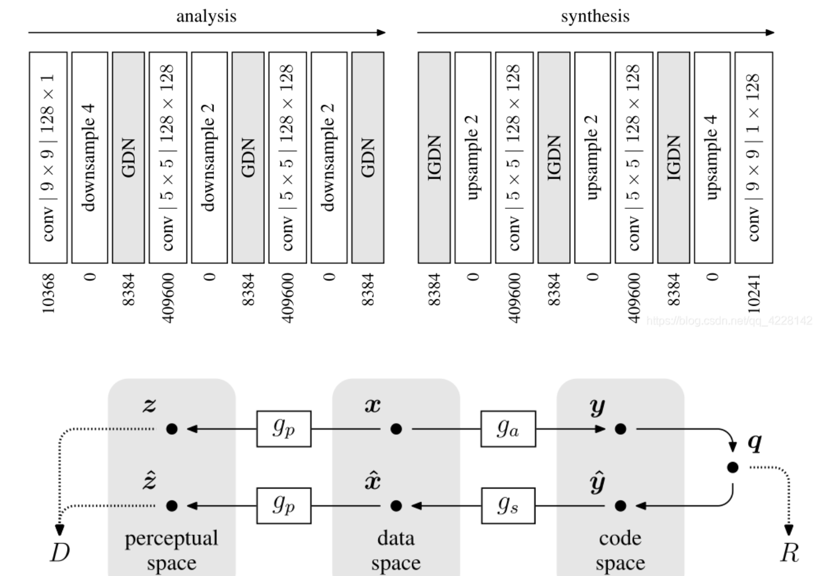
整体算法分为三个部分:非线性分析变换(编码器),均匀量化器和非线性合成边变换(解码器)
x 与 $\hat{x} $分别代表输入的原图和经过编解码器后的重建图片。
g a g_a ga表示编码器提供的非线性分析变换,即由输入图片经过编码器网络后得到的潜在特征,通过量化器q 后,得到 量化后结果:$ \hat{y} $
再通过 g S g_S gS解码器重建图片结果.
实践
TensorFlow Compression(TFC)是一个用于在TensorFlow中进行数据压缩和解压缩的库。它提供了一系列的压缩算法和工具,用于在机器学习和深度学习任务中对模型参数、特征和数据进行压缩。
使用TFC,你可以实现以下功能:
- 模型压缩:通过使用压缩算法对模型参数进行压缩,减少模型的存储空间和内存占用。
- 特征压缩:对输入数据的特征进行压缩,以减少特征的维度和表示大小。
- 数据压缩:对训练数据集或测试数据集进行压缩,以减少数据的存储和传输开销。
TFC提供了多种压缩算法,包括无损和有损压缩方法。其中一些常用的算法包括:
- GDN(Generalized Divisive Normalization):用于图像和视频数据的非线性特征压缩。
- Balle’s Method:一种基于无损压缩的算法,可用于对模型参数进行压缩。
- Entropy Coders:提供了各种熵编码器,如Arithmetic Coding和Huffman Coding,用于数据压缩。
通过使用TFC,你可以最大限度地减少模型和数据的存储空间,同时保持压缩后的数据的质量和准确性。这对于在资源受限的环境下部署机器学习模型或进行大规模数据处理非常有用。
学习网址 Learned data compression | TensorFlow Core
Overview
This notebook shows how to do lossy data compression using neural networks and TensorFlow Compression. Lossy compression involves making a trade-off between rate, the expected number of bits needed to encode a sample, and distortion, the expected error in the reconstruction of the sample. The examples below use an autoencoder-like model to compress images from the MNIST dataset.The method is based on the paper End-to-end Optimized Image Compression. More background on learned data compression can be found in this paper targeted at people familiar with classical data compression, or this survey targeted at a machine learning audience.
本笔记展示了如何使用神经网络和 TensorFlow Compression 进行有损数据压缩。 有损压缩涉及在速率(对样本进行编码所需的预期位数)和失真(样本重建中的预期误差)之间进行权衡。 下面的示例使用类似自动编码器的模型来压缩 MNIST 数据集中的图像。该方法基于论文“端到端优化图像压缩”。 有关学习数据压缩的更多背景信息可以在针对熟悉经典数据压缩的人员的本文或针对机器学习受众的调查中找到。
Define the trainer model
Because the model resembles an autoencoder, and we need to perform a different set of functions during training and inference, the setup is a little different from, say, a classifier.
The training model consists of three parts:
- the analysis (or encoder) transform, converting from the image into a latent space,
- the synthesis (or decoder) transform, converting from the latent space back into image space, and
- a prior and entropy model, modeling the marginal probabilities of the latents.
First, define the transforms:
由于该模型类似于自动编码器,并且我们需要在训练和推理期间执行一组不同的功能,因此设置与分类器等略有不同。 训练模型由三部分组成:
分析(或编码器)变换,从图像转换为潜在空间,
合成(或解码器)变换,从潜在空间转换回图像空间,
以及 先验和熵模型,对潜在的边际概率进行建模。
首先,定义变换:
def make_analysis_transform(latent_dims):"""Creates the analysis (encoder) transform."""return tf.keras.Sequential([tf.keras.layers.Conv2D(20, 5, use_bias=True, strides=2, padding="same",activation="leaky_relu", name="conv_1"),tf.keras.layers.Conv2D(50, 5, use_bias=True, strides=2, padding="same",activation="leaky_relu", name="conv_2"),tf.keras.layers.Flatten(),tf.keras.layers.Dense(500, use_bias=True, activation="leaky_relu", name="fc_1"),tf.keras.layers.Dense(latent_dims, use_bias=True, activation=None, name="fc_2"),], name="analysis_transform")
def make_synthesis_transform():"""Creates the synthesis (decoder) transform."""return tf.keras.Sequential([tf.keras.layers.Dense(500, use_bias=True, activation="leaky_relu", name="fc_1"),tf.keras.layers.Dense(2450, use_bias=True, activation="leaky_relu", name="fc_2"),tf.keras.layers.Reshape((7, 7, 50)),tf.keras.layers.Conv2DTranspose(20, 5, use_bias=True, strides=2, padding="same",activation="leaky_relu", name="conv_1"),tf.keras.layers.Conv2DTranspose(1, 5, use_bias=True, strides=2, padding="same",activation="leaky_relu", name="conv_2"),], name="synthesis_transform")
The trainer holds an instance of both transforms, as well as the parameters of the prior.
Its call method is set up to compute:
- rate, an estimate of the number of bits needed to represent the batch of digits, and
- distortion, the mean absolute difference between the pixels of the original digits and their reconstructions.
训练器保存两个变换的实例以及先验的参数。 其调用方法设置为计算:
速率,表示一批数字所需的位数的估计,
以及 失真,原始数字及其重建的像素之间的平均绝对差。
My idea:这里说的call就是下面代码中的call 方法,其作用是计算速率和失真
class MNISTCompressionTrainer(tf.keras.Model):"""Model that trains a compressor/decompressor for MNIST."""def __init__(self, latent_dims):super().__init__()self.analysis_transform = make_analysis_transform(latent_dims)self.synthesis_transform = make_synthesis_transform()self.prior_log_scales = tf.Variable(tf.zeros((latent_dims,)))@propertydef prior(self):return tfc.NoisyLogistic(loc=0., scale=tf.exp(self.prior_log_scales))def call(self, x, training):"""Computes rate and distortion losses."""# Ensure inputs are floats in the range (0, 1).x = tf.cast(x, self.compute_dtype) / 255.x = tf.reshape(x, (-1, 28, 28, 1))# Compute latent space representation y, perturb it and model its entropy,# then compute the reconstructed pixel-level representation x_hat.y = self.analysis_transform(x)entropy_model = tfc.ContinuousBatchedEntropyModel(self.prior, coding_rank=1, compression=False)y_tilde, rate = entropy_model(y, training=training)x_tilde = self.synthesis_transform(y_tilde)# Average number of bits per MNIST digit.rate = tf.reduce_mean(rate)# Mean absolute difference across pixels.distortion = tf.reduce_mean(abs(x - x_tilde))return dict(rate=rate, distortion=distortion)
My idea:计算潜空间表示y,对其进行扰动并建模其熵,然后计算重建的像素级表示x_hat。
Load the MNIST dataset for training and validation:
training_dataset, validation_dataset = tfds.load("mnist",split=["train", "test"],shuffle_files=True,as_supervised=True,with_info=False,
)
提取一张图像x
(x, _), = validation_dataset.take(1)plt.imshow(tf.squeeze(x))
print(f"Data type: {x.dtype}")
print(f"Shape: {x.shape}")
To get the latent representation y, we need to cast it to float32, add a batch dimension, and pass it through the analysis transform.
为了获得潜空间表示 y,我们需要将其转换为float32类型,添加批处理维度,并通过分析变换进行传递。
x = tf.cast(x, tf.float32) / 255.
x = tf.reshape(x, (-1, 28, 28, 1))
y = make_analysis_transform(10)(x)print("y:", y)
My idea:这里就是通过输入x(即图像)通过编码器来得到y
The latents will be quantized at test time. To model this in a differentiable way during training, we add uniform noise in the interval (−.5,.5) and call the result y ~ \widetilde y y . This is the same terminology as used in the paper End-to-end Optimized Image Compression.
y_tilde = y + tf.random.uniform(y.shape, -.5, .5)print("y_tilde:", y_tilde)
My idea:为了在量化的时候可微,加入了均匀噪声
The “prior” is a probability density that we train to model the marginal distribution of the noisy latents.For example, it could be a set of independent logistic distributions with different scales for each latent dimension.tfc.NoisyLogistic accounts for the fact that the latents have additive noise.As the scale approaches zero, a logistic distribution approaches a dirac delta (spike), but the added noise causes the “noisy” distribution to approach the uniform distribution instead.
“先验”是我们训练来模拟噪声潜伏的边缘分布的概率密度。例如,它可以是一组独立的逻辑分布,每个潜在维度具有不同的尺度。 tfc.NoisyLogistic 解释了潜在因素具有加性噪声的事实。当尺度接近零时,逻辑分布接近狄拉克三角洲(尖峰),但添加的噪声会导致“噪声”分布接近均匀分布。
prior = tfc.NoisyLogistic(loc=0., scale=tf.linspace(.01, 2., 10))_ = tf.linspace(-6., 6., 501)[:, None]
plt.plot(_, prior.prob(_));
During training, tfc.ContinuousBatchedEntropyModel adds uniform noise, and uses the noise and the prior to compute a (differentiable) upper bound on the rate (the average number of bits necessary to encode the latent representation).That bound can be minimized as a loss.
在训练期间,tfc.ContinouslyBatchedEntropyModel 添加均匀噪声,并使用噪声和先验来计算速率的(可微分)上限(编码潜在表示所需的平均位数)。该界限可以作为损失最小化。
entropy_model = tfc.ContinuousBatchedEntropyModel(prior, coding_rank=1, compression=False)
y_tilde, rate = entropy_model(y, training=True)print("rate:", rate)
print("y_tilde:", y_tilde)
Lastly, the noisy latents are passed back through the synthesis transform to produce an image reconstruction x ~ \widetilde x x . Distortion is the error between original image and reconstruction. Obviously, with the transforms untrained, the reconstruction is not very useful.
最后,将带有噪声的潜变量通过合成变换传递回去,生成图像重建x。失真是原始图像和重建图像之间的误差。显然,如果变换未经训练,重建图像是不太有用的。
x_tilde = make_synthesis_transform()(y_tilde)# Mean absolute difference across pixels.
distortion = tf.reduce_mean(abs(x - x_tilde))
print("distortion:", distortion)x_tilde = tf.saturate_cast(x_tilde[0] * 255, tf.uint8)
plt.imshow(tf.squeeze(x_tilde))
print(f"Data type: {x_tilde.dtype}")
print(f"Shape: {x_tilde.shape}")
For every batch of digits, calling the MNISTCompressionTrainer produces the rate and distortion as an average over that batch:
对于每批数字,调用 MNISTCompressionTrainer 会生成该批次的平均速率和失真:
(example_batch, _), = validation_dataset.batch(32).take(1)
trainer = MNISTCompressionTrainer(10)
example_output = trainer(example_batch)print("rate: ", example_output["rate"])
print("distortion: ", example_output["distortion"])
In the next section, we set up the model to do gradient descent on these two losses.
在下一节中,我们设置模型对这两个损失进行梯度下降。
My idea:没有量化吗,看下来好像就是一个图像直接扔近编码器,然后扔进熵编码,然后再通过解码器得到重建图
Train the model
We compile the trainer in a way that it optimizes the rate–distortion Lagrangian, that is, a sum of rate and distortion, where one of the terms is weighted by Lagrange parameter λ \lambda λ.
This loss function affects the different parts of the model differently:
- The analysis transform is trained to produce a latent representation that achieves the desired trade-off between rate and distortion.
- The synthesis transform is trained to minimize distortion, given the latent representation.
- The parameters of the prior are trained to minimize the rate given the latent representation. This is identical to fitting the prior to the marginal distribution of latents in a maximum likelihood sense.
My idea:编译训练器来优化速率-失真拉格朗日函数。
该损失函数对模型的不同部分产生不同的影响:
分析变换经过训练以产生潜在表示,从而实现速率和失真之间的所需权衡。
在给定潜在表示的情况下,训练合成变换以最小化失真。
先验参数的训练目标是在给定潜在表示的情况下最小化速率。从最大似然意义上说,这相当于将先验拟合到潜在表示的边缘分布 什么意思??????
def pass_through_loss(_, x):# Since rate and distortion are unsupervised, the loss doesn't need a target.# 由于速率和失真是无监督的,因此损失不需要目标。return xdef make_mnist_compression_trainer(lmbda, latent_dims=50):trainer = MNISTCompressionTrainer(latent_dims)trainer.compile(optimizer=tf.keras.optimizers.Adam(learning_rate=1e-3),# Just pass through rate and distortion as losses/metrics.# 只需将速率和失真作为损失/指标传递。loss=dict(rate=pass_through_loss, distortion=pass_through_loss),metrics=dict(rate=pass_through_loss, distortion=pass_through_loss),loss_weights=dict(rate=1., distortion=lmbda),)return trainer
Next, train the model.The human annotations are not necessary here, since we just want to compress the images, so we drop them using a map and instead add “dummy” targets for rate and distortion.
接下来,训练模型。这里不需要人工注释,因为我们只想压缩图像,所以我们使用字典删除它们,而是添加速率和失真的“虚拟”目标。
def add_rd_targets(image, label):# Training is unsupervised, so labels aren't necessary here. However, we# need to add "dummy" targets for rate and distortion.return image, dict(rate=0., distortion=0.)def train_mnist_model(lmbda):trainer = make_mnist_compression_trainer(lmbda)trainer.fit(training_dataset.map(add_rd_targets).batch(128).prefetch(8),epochs=15,validation_data=validation_dataset.map(add_rd_targets).batch(128).cache(),validation_freq=1,verbose=1,)return trainertrainer = train_mnist_model(lmbda=2000)
Compress some MNIST images
For compression and decompression at test time, we split the trained model in two parts:
- The encoder side consists of the analysis transform and the entropy model.
- The decoder side consists of the synthesis transform and the same entropy model.
At test time, the latents will not have additive noise, but they will be quantized and then losslessly compressed, so we give them new names. We call them and the image reconstruction x ^ \hat x x^ and y ^ \hat y y^, respectively (following End-to-end Optimized Image Compression).
class MNISTCompressor(tf.keras.Model):"""Compresses MNIST images to strings."""def __init__(self, analysis_transform, entropy_model):super().__init__()self.analysis_transform = analysis_transformself.entropy_model = entropy_modeldef call(self, x):# Ensure inputs are floats in the range (0, 1).x = tf.cast(x, self.compute_dtype) / 255.y = self.analysis_transform(x)# Also return the exact information content of each digit._, bits = self.entropy_model(y, training=False)return self.entropy_model.compress(y), bits
class MNISTDecompressor(tf.keras.Model):"""Decompresses MNIST images from strings."""def __init__(self, entropy_model, synthesis_transform):super().__init__()self.entropy_model = entropy_modelself.synthesis_transform = synthesis_transformdef call(self, string):y_hat = self.entropy_model.decompress(string, ())x_hat = self.synthesis_transform(y_hat)# Scale and cast back to 8-bit integer.return tf.saturate_cast(tf.round(x_hat * 255.), tf.uint8)
When instantiated with compression=True, the entropy model converts the learned prior into tables for a range coding algorithm.When calling compress(), this algorithm is invoked to convert the latent space vector into bit sequences.The length of each binary string approximates the information content of the latent (the negative log likelihood of the latent under the prior).
The entropy model for compression and decompression must be the same instance, because the range coding tables need to be exactly identical on both sides.Otherwise, decoding errors can occur.
当使用compression = True 进行实例化时,熵模型将学习到的先验转换为范围编码算法的表。当调用 compress() 时,会调用该算法将潜在空间向量转换为位序列。每个二进制字符串的长度近似于潜在的信息内容(潜在在先验条件下的负对数似然)。
压缩和解压缩的熵模型必须是相同的实例,因为范围编码表需要两侧完全相同。否则,可能会发生解码错误。
def make_mnist_codec(trainer, **kwargs):# The entropy model must be created with `compression=True` and the same# instance must be shared between compressor and decompressor.entropy_model = tfc.ContinuousBatchedEntropyModel(trainer.prior, coding_rank=1, compression=True, **kwargs)compressor = MNISTCompressor(trainer.analysis_transform, entropy_model)decompressor = MNISTDecompressor(entropy_model, trainer.synthesis_transform)return compressor, decompressorcompressor, decompressor = make_mnist_codec(trainer)
Grab 16 images from the validation dataset.You can select a different subset by changing the argument to skip
从验证数据集中获取 16 张图像。您可以通过更改跳过参数来选择不同的子集
(originals, _), = validation_dataset.batch(16).skip(3).take(1)
Compress them to strings, and keep track of each of their information content in bits.
将它们压缩为字符串,并以位的形式跟踪它们的每个信息内容。
strings, entropies = compressor(originals)print(f"String representation of first digit in hexadecimal: 0x{strings[0].numpy().hex()}")
print(f"Number of bits actually needed to represent it: {entropies[0]:0.2f}")
Decompress the images back from the strings.
将图像从字符串中解压回来。
reconstructions = decompressor(strings)
Display each of the 16 original digits together with its compressed binary representation, and the reconstructed digit.
显示 16 个原始数字中的每一个及其压缩的二进制表示形式,以及重建的数字。
def display_digits(originals, strings, entropies, reconstructions):"""Visualizes 16 digits together with their reconstructions."""fig, axes = plt.subplots(4, 4, sharex=True, sharey=True, figsize=(12.5, 5))axes = axes.ravel()for i in range(len(axes)):image = tf.concat([tf.squeeze(originals[i]),tf.zeros((28, 14), tf.uint8),tf.squeeze(reconstructions[i]),], 1)axes[i].imshow(image)axes[i].text(.5, .5, f"→ 0x{strings[i].numpy().hex()} →\n{entropies[i]:0.2f} bits",ha="center", va="top", color="white", fontsize="small",transform=axes[i].transAxes)axes[i].axis("off")plt.subplots_adjust(wspace=0, hspace=0, left=0, right=1, bottom=0, top=1)
display_digits(originals, strings, entropies, reconstructions)
Note that the length of the encoded string differs from the information content of each digit.
This is because the range coding process works with discrete probabilities, and has a small amount of overhead. So, especially for short strings, the correspondence is only approximate. However, range coding is asymptotically optimal: in the limit, the expected bit count will approach the cross entropy (the expected information content), for which the rate term in the training model is an upper bound.
请注意,编码字符串的长度与每个数字的信息内容不同。
这是因为范围编码过程使用离散概率,并且具有少量开销。因此,特别是对于短字符串,对应关系只是近似的。然而,范围编码是渐近最优的:在极限情况下,预期的比特数将接近交叉熵(预期的信息内容),其中训练模型中的速率项是上限。
The rate–distortion trade-off
率与失真的权衡
Above, the model was trained for a specific trade-off (given by lmbda=2000) between the average number of bits used to represent each digit and the incurred error in the reconstruction.
What happens when we repeat the experiment with different values?
Let’s start by reducing λ \lambda λ to 500.
在上述例子中,模型是根据给定的权衡(由lmbda=2000确定)在表示每个数字所使用的平均比特数和重建时产生的误差之间进行训练的。
当我们使用不同的值重复实验时会发生什么呢?
def train_and_visualize_model(lmbda):trainer = train_mnist_model(lmbda=lmbda)compressor, decompressor = make_mnist_codec(trainer)strings, entropies = compressor(originals)reconstructions = decompressor(strings)display_digits(originals, strings, entropies, reconstructions)train_and_visualize_model(lmbda=500)
The strings begin to get much shorter now, on the order of one byte per digit.However, this comes at a cost.More digits are becoming unrecognizable.
This demonstrates that this model is agnostic to human perceptions of error, it just measures the absolute deviation in terms of pixel values.To achieve a better perceived image quality, we would need to replace the pixel loss with a perceptual loss.
现在字符串开始变得更短,大约每个数字一个字节。然而,这是有代价的。更多的数字变得无法识别。
这表明该模型与人类对错误的感知无关,它仅测量像素值的绝对偏差。为了获得更好的感知图像质量,我们需要用感知损失来代替像素损失。
Use the decoder as a generative model
使用解码器作为生成模型
If we feed the decoder random bits, this will effectively sample from the distribution that the model learned to represent digits.
First, re-instantiate the compressor/decompressor without a sanity check that would detect if the input string isn’t completely decoded.
如果我们向解码器提供随机位,这将有效地从模型学习表示数字的分布中进行采样。 首先,重新实例化压缩器/解压缩器,而不进行健全性检查,以检测输入字符串是否未完全解码。
compressor, decompressor = make_mnist_codec(trainer, decode_sanity_check=False)
Now, feed long enough random strings into the decompressor so that it can decode/sample digits from them.
现在,将足够长的随机字符串输入解压缩器,以便它可以解码/采样其中的数字。
import osstrings = tf.constant([os.urandom(8) for _ in range(16)])
samples = decompressor(strings)fig, axes = plt.subplots(4, 4, sharex=True, sharey=True, figsize=(5, 5))
axes = axes.ravel()
for i in range(len(axes)):axes[i].imshow(tf.squeeze(samples[i]))axes[i].axis("off")
plt.subplots_adjust(wspace=0, hspace=0, left=0, right=1, bottom=0, top=1)
tensorflow.python.framework.errors_impl.NotFoundError: /home/jjh/compression-master/tensorflow_compression/python/ops/…/…/cc/libtensorflow_compression.so: cannot open shared object file:


cd tensorflow_compression
python -m pip install -U pip setuptools wheel
变分自编码器
通过 tf.keras.Sequential 连接生成网络与推理网络
在此 VAE 示例中,对编码器和解码器网络使用两个小型 ConvNet。在文献中,这些网络也分别称为推断/识别和生成模型。使用 tf.keras.Sequential 来简化实现。在下面的描述中,使 x 和 z 分别表示观测值和隐变量。
生成网络
这定义了近似后验分布 q(z|x),它会将输入取作观测值并输出一组参数,用于指定隐变量表示 z 的条件分布。在本例中,简单地将分布建模为对角高斯分布,网络会输出分解高斯分布的均值和对数方差参数。输出对数方差而不是直接用于数值稳定性的方差。
推理网络
这定义了观测值的条件分布 p(x|z),它会将隐变量样本 z 取作输入并输出观测值条件分布的参数。将隐变量先验分布 p(z) 建模为单位高斯分布。
重参数化技巧
要在训练期间为解码器生成样本 z,您可以在给定输入观测值 x 的情况下从编码器输出的参数所定义的隐变量分布中采样。然而,这种采样操作会产生瓶颈,因为反向传播不能流经随机节点。
要解决这个问题,请使用重参数化技巧。在我们的示例中,使用解码器参数 ε \varepsilon ε和另一个参数 来逼近 z,如下所示:
z = μ + σ ∗ ε z=\mu+\sigma *\varepsilon z=μ+σ∗ε
其中 μ \mu μ 和 σ \sigma σ 分别代表高斯分布的均值和标准差。它们可通过解码器输出推导得出。 ε \varepsilon ε可被认为是用于保持 z 的随机性的随机噪声。从标准正态分布生成 ε \varepsilon ε。
隐变量 z 现在由 μ \mu μ 、 σ \sigma σ 和 ε \varepsilon ε的函数生成,这将使模型能够分别通过$ \mu$ 和 σ \sigma σ在编码器中反向传播梯度,同时通过$ \varepsilon $保持随机性。
网络架构
对于编码器网络,使用两个卷积层后接一个全连接层。在解码器网络中,通过使用一个全连接层后接三个卷积转置层(在某些背景下也称为反卷积层)来镜像此架构。请注意,通常的做法是在训练 VAE 时避免使用批量归一化,因为使用 mini-batch 导致的额外随机性可能会在提高采样随机性的同时加剧不稳定性。
