DCGAN整理总结
- GAN
- 什么是GAN?
- GAN重要参数及损失函数
- DCGAN
- 什么是DCGAN?
- DCGAN结构
- TensorFlow版本MINIST手写体生成模型
- Pytorch版本人脸生成模型
GAN
什么是GAN?
GAN是一个教深度学习模型捕捉训练数据的布局来从该布局中生成新数据的框架。最早是2014年Ian Goodfellow提出的。GAN主要由两部分模型组成——生成器和判别器。
生成器的工作是生成极像训练数据的“假”数据,判别器的工作是判断一张照片是一个真实的训练照片还是生成器生成的假照片。训练时,生成器尝试生成越来越好的假照片来欺骗判别器,而判别器不断更好的发现和正确辨别真实的和假冒的照片。
博弈的平衡点是当生成器生成的伪造品看起来像直接来自训练数据时,而鉴别器则总是猜测生成器输出是真实还是伪造品的置信度为50%。
GAN重要参数及损失函数
由于是处理图像,输入判别器的图像大小为CHW:3X64X64
x:图像的数据表征
D(x):判别器输出的判断x来自真实训练数据的可能性(当x来自真实训练集,该值应该偏大,当x为生成器生成的,则该值应该偏小)可以看做是一个传统的二分类
z:是一个从标准正态分布中抽样的隐空间向量
G(z):表示生成器从隐向量z映射到数据空间的函数(G的目的是估计训练数据来自的分布(pdata),从而可以从**估计的分布(pg)**中生成假的样本)
D(G(z)):是判断生成器G的输出是一个真实图像的概率。
实际上,D和G在玩一个minimax游戏,D尽力去最大化正确区分真假的概率(logD(x)),G尽力去最小化D预测G的输出是假的的概率(log(1−D(G(x))))。
从而得出GAN的损失函数:
minGmaxD V(D,G)=Ex~pdata(x)[logD(x)]+Ez~pz(z)[log(1−D(G(z)))]
理论上说,这个minimax游戏的最终结果是pg=pdata,并且判别器是随机猜测输入是真或假。
实际上,该收敛理论仍在积极研究中,模型并不总是能达到该目的。
DCGAN
什么是DCGAN?
深度学习中对图像处理应用最好的模型是CNN,DCGAN是把CNN与GAN相结合的一次尝试。
DCGAN与GAN的原理是一样的,只是把D和G换成了两个卷积神经网络。但并不是直接替换,而是对卷积神经网络结构做了一些改变,来提高样本质量和收敛速度。
DCGAN结构

主要有以下改变:
- 取消所有pooling层。G网络中使用转置卷积(transposed convolutional layer)进行上采样,D网络中用加入stride的卷积代替pooling。
- 在D和G中均使用batch normalization(批归范化)
- 去掉FC(全连接)层,使网络变为全卷积网络
- G网络中使用ReLU作为激活函数,最后一层使用tanh
- D网络中使用LeakyReLU作为激活函数
TensorFlow版本MINIST手写体生成模型
以下内容摘自:https://www.tensorflow.org/tutorials/generative/dcgan
导入TensorFlow和其他包:
import tensorflow as tf
import glob
import imageio
import matplotlib.pyplot as plt
import numpy as np
import os
import PIL
from tensorflow.keras import layers
import timefrom IPython import displaytf.__version__
# '2.3.0'
# 用于生成 GIF 图片
pip install -q imageio
加载和准备数据集:
(train_images, train_labels), (_, _) = f.keras.datasets.mnist.load_data()
train_images = train_images.reshape(train_images.shape[0], 28, 28, 1).astype('float32')
train_images = (train_images - 127.5) / 127.5 # 将图片标准化到 [-1, 1] 区间内
BUFFER_SIZE = 60000
BATCH_SIZE = 256
# 批量化和打乱数据
train_dataset = tf.data.Dataset.from_tensor_slices(train_images).shuffle(BUFFER_SIZE).batch(BATCH_SIZE)
生成器结构:
def make_generator_model():# 定义一个序列模型model = tf.keras.Sequential() # 添加一个全连接层:输入为一个7*7*256的随机种子,不使用偏置项,设置输入大小为100维度。model.add(layers.Dense(7*7*256, use_bias=False, input_shape=(100,)))# 添加批处理规范化,加速训练平稳收敛model.add(layers.BatchNormalization()) # 是ReLU激活函数的变体,对负值输入有很小的坡度,导数总是不为0,从而减少静默神经元的出现。model.add(layers.LeakyReLU()) # 重塑层的形状model.add(layers.Reshape((7, 7, 256))) assert model.output_shape == (None, 7, 7, 256) # 添加反卷积层,输出维度128,卷积核大小为5*5,步长为1model.add(layers.Conv2DTranspose(128, (5, 5), strides=(1, 1), padding='same', use_bias=False))assert model.output_shape == (None, 7, 7, 128)model.add(layers.BatchNormalization())model.add(layers.LeakyReLU())# 添加反卷积层,输出维度64,卷积核大小为5*5,步长为2model.add(layers.Conv2DTranspose(64, (5, 5), strides=(2, 2), padding='same', use_bias=False))assert model.output_shape == (None, 14, 14, 64)model.add(layers.BatchNormalization())model.add(layers.LeakyReLU())# 添加反卷积层,输出维度1,卷积核大小为5*5,步长为2model.add(layers.Conv2DTranspose(1, (5, 5), strides=(2, 2), padding='same', use_bias=False, activation='tanh'))assert model.output_shape == (None, 28, 28, 1)return model
使用未训练的生成器产生一张图片。
generator = make_generator_model()noise = tf.random.normal([1, 100])
generated_image = generator(noise, training=False)plt.imshow(generated_image[0, :, :, 0], cmap='gray')

判别器结构:
def make_discriminator_model():# 创建序列模型model = tf.keras.Sequential()# 之前的反过程:先添加一个卷积层,输出维度为64,卷积核大小5*5,步长为2,输入为28*28*1大小图片model.add(layers.Conv2D(64, (5, 5), strides=(2, 2), padding='same',input_shape=[28, 28, 1]))model.add(layers.LeakyReLU())# 添加dropout层防止过拟合model.add(layers.Dropout(0.3))# 添加一个卷积层,输出维度128,卷积核大小5*5,步长为2model.add(layers.Conv2D(128, (5, 5), strides=(2, 2), padding='same'))model.add(layers.LeakyReLU())model.add(layers.Dropout(0.3))# 添加扁平层,即把多维的输入一维化,常用在从卷积层到全连接层的过渡。model.add(layers.Flatten())# 定义全连接层,输出维度为1model.add(layers.Dense(1))return model使用(尚未训练的)判别器来对图片的真伪进行判断。模型将被训练为为真实图片输出正值,为伪造图片输出负值。
discriminator = make_discriminator_model()
decision = discriminator(generated_image)
print (decision)
#tf.Tensor([[-0.00427552]], shape=(1, 1), dtype=float32)
定义损失函数和优化器:
# 该方法返回计算交叉熵损失的辅助函数,采用的是sigmoid+交叉熵函数
cross_entropy = tf.keras.losses.BinaryCrossentropy(from_logits=True)
判别器损失:
该方法量化判别器从判断真伪图片的能力。它将判别器对真实图片的预测值与值全为 1 的数组进行对比,将判别器对伪造(生成的)图片的预测值与值全为 0 的数组进行对比。
def discriminator_loss(real_output, fake_output):real_loss = cross_entropy(tf.ones_like(real_output), real_output)fake_loss = cross_entropy(tf.zeros_like(fake_output), fake_output)total_loss = real_loss + fake_lossreturn total_loss
生成器损失:
生成器损失量化其欺骗判别器的能力。直观来讲,如果生成器表现良好,判别器将会把伪造图片判断为真实图片(或 1)。这里我们将把判别器在生成图片上的判断结果与一个值全为 1 的数组进行对比。
def generator_loss(fake_output):return cross_entropy(tf.ones_like(fake_output), fake_output)
优化器:
generator_optimizer = tf.keras.optimizers.Adam(1e-4)
discriminator_optimizer = tf.keras.optimizers.Adam(1e-4)
保存检查点:
checkpoint_dir = './training_checkpoints'
checkpoint_prefix = os.path.join(checkpoint_dir, "ckpt")
checkpoint = tf.train.Checkpoint(generator_optimizer=generator_optimizer,discriminator_optimizer=discriminator_optimizer,generator=generator,discriminator=discriminator)
定义训练循环:
EPOCHS = 50
noise_dim = 100
num_examples_to_generate = 16# 我们将重复使用该种子(因此在动画 GIF 中更容易可视化进度)
seed = tf.random.normal([num_examples_to_generate, noise_dim])
训练循环在生成器接收到一个随机种子作为输入时开始。该种子用于生产一张图片。判别器随后被用于区分真实图片(选自训练集)和伪造图片(由生成器生成)。针对这里的每一个模型都计算损失函数,并且计算梯度用于更新生成器与判别器。
# 注意 `tf.function` 的使用
# 该注解使函数被“编译”
@tf.function
def train_step(images):noise = tf.random.normal([BATCH_SIZE, noise_dim]) # 随机噪声with tf.GradientTape() as gen_tape, tf.GradientTape() as disc_tape:generated_images = generator(noise, training=True)real_output = discriminator(images, training=True)fake_output = discriminator(generated_images, training=True)gen_loss = generator_loss(fake_output)disc_loss = discriminator_loss(real_output, fake_output)gradients_of_generator = gen_tape.gradient(gen_loss, generator.trainable_variables)gradients_of_discriminator = disc_tape.gradient(disc_loss, discriminator.trainable_variables)generator_optimizer.apply_gradients(zip(gradients_of_generator, generator.trainable_variables))discriminator_optimizer.apply_gradients(zip(gradients_of_discriminator, discriminator.trainable_variables))
def train(dataset, epochs):for epoch in range(epochs):start = time.time()for image_batch in dataset:train_step(image_batch)# 继续进行时为 GIF 生成图像display.clear_output(wait=True)generate_and_save_images(generator,epoch + 1,seed)# 每 15 个 epoch 保存一次模型if (epoch + 1) % 15 == 0:checkpoint.save(file_prefix = checkpoint_prefix)print ('Time for epoch {} is {} sec'.format(epoch + 1, time.time()-start))# 最后一个 epoch 结束后生成图片display.clear_output(wait=True)generate_and_save_images(generator,epochs,seed)
生成与保存照片:
def generate_and_save_images(model, epoch, test_input):# 注意 training` 设定为 False# 因此,所有层都在推理模式下运行(batchnorm)。predictions = model(test_input, training=False)fig = plt.figure(figsize=(4,4))for i in range(predictions.shape[0]):plt.subplot(4, 4, i+1)plt.imshow(predictions[i, :, :, 0] * 127.5 + 127.5, cmap='gray')plt.axis('off')plt.savefig('image_at_epoch_{:04d}.png'.format(epoch))plt.show()
训练模型:
调用上面定义的 train() 方法来同时训练生成器和判别器。注意,训练 GANs 可能是棘手的。重要的是,生成器和判别器不能够互相压制对方(例如,他们以相似的学习率训练)。
在训练之初,生成的图片看起来像是随机噪声。随着训练过程的进行,生成的数字将越来越真实。在大概 50 个 epoch 之后,这些图片看起来像是 MNIST 数字。使用 Colab 中的默认设置可能需要大约 1 分钟每 epoch。
%%time
train(train_dataset, EPOCHS)

恢复检查点:
checkpoint.restore(tf.train.latest_checkpoint(checkpoint_dir))
生成gif动画:
# 使用 epoch 数生成单张图片
def display_image(epoch_no):return PIL.Image.open('image_at_epoch_{:04d}.png'.format(epoch_no))
display_image(EPOCHS)
anim_file = 'dcgan.gif'with imageio.get_writer(anim_file, mode='I') as writer:filenames = glob.glob('image*.png')filenames = sorted(filenames)last = -1for i,filename in enumerate(filenames):frame = 2*(i**0.5)if round(frame) > round(last):last = frameelse:continueimage = imageio.imread(filename)writer.append_data(image)image = imageio.imread(filename)writer.append_data(image)import IPython
if IPython.version_info > (6,2,0,''):display.Image(filename=anim_file)
如果使用colab执行代码,可用以下代码保存gif图像:
try:from google.colab import files
except ImportError:pass
else:files.download(anim_file)

Pytorch版本人脸生成模型
以下内容摘自:https://pytorch.org/tutorials/beginner/dcgan_faces_tutorial.html
注:该模型对上图中的DCGAN结构有所改动,第一个转置卷积调整通道数变为512,非1024。
引入需要的包:
# 在开头加上这句之后,即使在python2.X,使用print也得像python3.X那样加括号使用。
from __future__ import print_function#%matplotlib inline
# argsparse是python的命令行解析的标准模块,内置于python,不需要安装。
# 这个库可以让我们直接在命令行中就可以向程序中传入参数并让程序运行。
import argparse
# 针对操作系统的包
import os
# 主要用于生成随机数
import random
# pytorch框架的库
import torch
# 主要包含了用来搭建各个层的模块(Modules),比如全连接、二维卷积、池化等,还有一些损失函数。
import torch.nn as nn
# 并行计算,执行多GPU计算
import torch.nn.parallel
# cuDNN使用非确定性算法,并且可以使用torch.backends.cudnn.enabled = False来进行禁用
import torch.backends.cudnn as cudnn
# torch.optim是一个实现了各种优化算法的库。
import torch.optim as optim
# 主要使用其中表示Dataset的抽象类
import torch.utils.data
# 包含了数据集:MNIST、COCO(用于图像标注和目标检测)、LSUN Classification、ImageFolder(通用的数据加载器)
# Imagenet-12、CIFAR10 and CIFAR100、STL10,它们都是上面类的子类。
import torchvision.datasets as dset
# 主要作用是对PIL.Image进行变换
import torchvision.transforms as transforms
# 处理图片的工具库,make_grid函数将图片排列成网格状
import torchvision.utils as vutils
# 数值计算的库
import numpy as np
# 是matplotlib的基于状态的接口,主要用于画图
import matplotlib.pyplot as plt
# 主要用于动画生成/画动态图
import matplotlib.animation as animation
# 包含8个主要函数,用于显示图片等
from IPython.display import HTML# Set random seed for reproducibility
manualSeed = 999
#manualSeed = random.randint(1, 10000) # use if you want new results
print("Random Seed: ", manualSeed)
random.seed(manualSeed) # seed()方法改变随机数生成器的种子,可以在调用其他随机模块函数之前调用此函数
torch.manual_seed(manualSeed) # 设置 (CPU) 生成随机数的种子,并返回一个torch.Generator对象。设置种子的用意是一旦固定种子,后面依次生成的随机数其实都是固定的。
定义输入项:
# Root directory for dataset 数据集文件夹根目录路径
dataroot = "data/celeba"# Number of workers for dataloader 用dataloader加载数据的工作线程数为2
workers = 2# Batch size during training 训练批次的大小为128
batch_size = 128# Spatial size of training images. All images will be resized to this
#   size using a transformer. 训练图像的空间大小,所有的图像都会通过转换器转换为该大小。
image_size = 64# Number of channels in the training images. For color images this is 3 训练图像的通道数为3
nc = 3# Size of z latent vector (i.e. size of generator input) 隐向量的长度/生成器输入的大小为100
nz = 100# Size of feature maps in generator 生成器特征图大小为64
ngf = 64# Size of feature maps in discriminator 判别器特征图大小为64
ndf = 64# Number of training epochs 训练迭代次数为5
num_epochs = 5# Learning rate for optimizers 优化器学习率为0.0002
lr = 0.0002# Beta1 hyperparam for Adam optimizers adam优化器中的beta1参数设置为0.5
beta1 = 0.5# Number of GPUs available. Use 0 for CPU mode. 可用的GPU数量,为1,为0时使用CPU
ngpu = 1
加载数据集:
数据来源:Google Drive https://drive.google.com/drive/folders/0B7EVK8r0v71pTUZsaXdaSnZBZzg
使用ImageFolder数据集类,它要求在数据集的根文件夹中有子目录。创建数据集,创建数据加载器,设置要运行的设备,最后可视化一些训练数据。
# We can use an image folder dataset the way we have it setup.
# Create the dataset 依据文件数据创建数据集(预处理图像)
dataset = dset.ImageFolder(root=dataroot,transform=transforms.Compose([transforms.Resize(image_size), # 统一大小transforms.CenterCrop(image_size), # 从中心位置裁剪transforms.ToTensor(), # 把灰度范围从0-255变换到0-1之间transforms.Normalize((0.5, 0.5, 0.5), (0.5, 0.5, 0.5)), # 把0-1变换到(-1,1)]))
# Create the dataloader 创建数据加载器,结合了数据集和取样器,并且可以提供多个线程处理数据集。
dataloader = torch.utils.data.DataLoader(dataset, batch_size=batch_size,shuffle=True, num_workers=workers)# Decide which device we want to run on
"""这段代码一般写在读取数据之前,torch.device代表将torch.Tensor分配到的设备的对象。
torch.device包含一个设备类型(‘cpu’或‘cuda’)和可选的设备序号。如果设备序号不存在,则为当前设备。
如:torch.Tensor用设备构建‘cuda’的结果等同于‘cuda:X’,其中X是torch.cuda.current_device()的结果。"""
print(torch.cuda.is_available())device = torch.device("cuda:0" if (torch.cuda.is_available() and ngpu > 0) else "cpu")# Plot some training images
#real_batch是一个列表
#第一个元素real_batch[0]是[128,3,64,64]的tensor,就是标准的一个batch的4D结构:128张图,3个通道,64长,64宽
#第二个元素real_batch[1]是第一个元素的标签,有128个label值全为0
real_batch = next(iter(dataloader)) # 生成迭代器并获取第一批次的图片集
plt.figure(figsize=(8,8)) # 定义图像大小为8*8
plt.axis("off") # 关闭坐标刻度
plt.title("Training Images") # 图像标题
plt.imshow(np.transpose(vutils.make_grid(real_batch[0].to(device)[:64], padding=2, normalize=True).cpu(),(1,2,0)))

权重初始化:
在DCGAN的论文中,作者规定所有模型权重应随机从均值为0,标准偏差为0.02的正态分布中初始化。“weights_init”函数将初始化的模型作为输入,并重新初始化所有卷积、卷积转置和批处理规范化层,以满足此标准。此函数在初始化后立即应用于模型。
def weights_init(m):classname = m.__class__.__name__if classname.find('Conv') != -1:nn.init.normal_(m.weight.data, 0.0, 0.02)elif classname.find('BatchNorm') != -1:nn.init.normal_(m.weight.data, 1.0, 0.02)nn.init.constant_(m.bias.data, 0)
生成器结构:
class Generator(nn.Module):def __init__(self, ngpu): # ngpu为GPU数量super(Generator, self).__init__()self.ngpu = ngpu# 定义序列模型self.main = nn.Sequential(# input is Z, going into a convolution# 添加反卷积层,输入通道数为100,输出通道数为64*8,卷积核大小为4*4,步长为1,padding为0nn.ConvTranspose2d( nz, ngf * 8, 4, 1, 0, bias=False),# 批处理标准化,该函数输入为卷积层输出通道数。nn.BatchNorm2d(ngf * 8),
# 设置激活函数为relunn.ReLU(True),# state size. (ngf*8) x 4 x 4# 添加反卷积层,输入通道数为64*8,输出通道数为64*4,卷积核大小为4*4,步长为2,padding为1nn.ConvTranspose2d(ngf * 8, ngf * 4, 4, 2, 1, bias=False),nn.BatchNorm2d(ngf * 4),nn.ReLU(True),# state size. (ngf*4) x 8 x 8# 添加反卷积层,输入通道数为64*4,输出通道数为64*2,卷积核大小为4*4,步长为2,padding为1nn.ConvTranspose2d( ngf * 4, ngf * 2, 4, 2, 1, bias=False),nn.BatchNorm2d(ngf * 2),nn.ReLU(True),# state size. (ngf*2) x 16 x 16# 添加反卷积层,输入通道数为64*2,输出通道数为64,卷积核大小为4*4,步长为2,padding为1nn.ConvTranspose2d( ngf * 2, ngf, 4, 2, 1, bias=False),nn.BatchNorm2d(ngf),nn.ReLU(True),# state size. (ngf) x 32 x 32# 添加反卷积层,输入通道数为64,输出通道数为3,卷积核大小为4*4,步长为2,padding为1nn.ConvTranspose2d( ngf, nc, 4, 2, 1, bias=False),#最后使用tanh作为激活函数nn.Tanh()# state size. (nc) x 64 x 64)def forward(self, input):return self.main(input)
实例化生成器:
# Create the generator
netG = Generator(ngpu).to(device)# Handle multi-gpu if desired
if (device.type == 'cuda') and (ngpu > 1):netG = nn.DataParallel(netG, list(range(ngpu)))# Apply the weights_init function to randomly initialize all weights
#  to mean=0, stdev=0.2.
netG.apply(weights_init)# Print the model
print(netG)

判别器结构:
class Discriminator(nn.Module):def __init__(self, ngpu):super(Discriminator, self).__init__()self.ngpu = ngpu# 定义序列模型self.main = nn.Sequential(# 是上面过程的反过程# input is (nc) x 64 x 64# 添加卷积层,输入通道数为3,输出通道数为64,卷积核大小4*4,步长2,padding为1 nn.Conv2d(nc, ndf, 4, 2, 1, bias=False),# leakyrelu作为激活函数nn.LeakyReLU(0.2, inplace=True),# state size. (ndf) x 32 x 32# 添加卷积层,输入通道数为64,输出通道数为64*2,卷积核大小4*4,步长2,padding为1 nn.Conv2d(ndf, ndf * 2, 4, 2, 1, bias=False),nn.BatchNorm2d(ndf * 2),nn.LeakyReLU(0.2, inplace=True),# state size. (ndf*2) x 16 x 16# 添加卷积层,输入通道数为64*2,输出通道数为64*4,卷积核大小4*4,步长2,padding为1 nn.Conv2d(ndf * 2, ndf * 4, 4, 2, 1, bias=False),nn.BatchNorm2d(ndf * 4),nn.LeakyReLU(0.2, inplace=True),# state size. (ndf*4) x 8 x 8# 添加卷积层,输入通道数为64*4,输出通道数为64*8,卷积核大小4*4,步长2,padding为1 nn.Conv2d(ndf * 4, ndf * 8, 4, 2, 1, bias=False),nn.BatchNorm2d(ndf * 8),nn.LeakyReLU(0.2, inplace=True),# state size. (ndf*8) x 4 x 4# 添加卷积层,输入通道数为64*8,输出通道数为1,卷积核大小4*4,步长1,padding为0 nn.Conv2d(ndf * 8, 1, 4, 1, 0, bias=False),# 最终以sigmoid作为激活函数nn.Sigmoid())def forward(self, input):return self.main(input)
实例化判别器:
# Create the Discriminator
netD = Discriminator(ngpu).to(device)# Handle multi-gpu if desired
if (device.type == 'cuda') and (ngpu > 1):netD = nn.DataParallel(netD, list(range(ngpu)))# Apply the weights_init function to randomly initialize all weights
#  to mean=0, stdev=0.2.
netD.apply(weights_init)# Print the model
print(netD)

损失函数和优化器:
D和G准备好后,我们可以指定它们如何通过损失函数和优化器进行学习。我们将使用pytorch中定义的二进制交叉熵损失(BECloss)函数:
ℓ(x,y)=L={l1,…,lN}⊤,ln=−[yn⋅logxn+(1−yn)⋅log(1−xn)]
注意该函数如何提供目标函数中两个组件的计算(即 log(D(x)) 和 log(1−D(G(z))))。我们可以指定BCE方程的哪一部分使用y作为输入。这是在即将到来的训练循环中完成的,但重要的是要了解如何通过改变y(即GT标签)来选择要计算的组件。
接下来,我们将真标签定义为1,假标签定义为0。在计算损失时,也将使用原始的G和G。最后,我们设置了两个独立的优化器,一个用于D,一个用于G。如DCGAN论文中所述,这两个都是Adam优化器,学习率为0.0002,Beta1=0.5。为了跟踪生成器的学习进程,我们将从高斯分布(即固定噪声)中生成一批固定的潜在向量。在训练循环中,我们将周期性地将这个固定噪声输入G中,在迭代过程中,我们将看到由噪声形成的图像。
# Initialize BCELoss function
criterion = nn.BCELoss()# Create batch of latent vectors that we will use to visualize
#  the progression of the generator
fixed_noise = torch.randn(64, nz, 1, 1, device=device)# Establish convention for real and fake labels during training
real_label = 1.
fake_label = 0.# Setup Adam optimizers for both G and D
optimizerD = optim.Adam(netD.parameters(), lr=lr, betas=(beta1, 0.999))
optimizerG = optim.Adam(netG.parameters(), lr=lr, betas=(beta1, 0.999))
训练:
我们将“构造不同的小批量的真假图像”,并调整G的目标函数以使logD(G(z))最大化。训练分为两个主要部分。第1部分更新了鉴别器,第2部分更新了生成器。
# Training Loop# Lists to keep track of progress
img_list = []
G_losses = []
D_losses = []
iters = 0print(device)print("Starting Training Loop...")
# For each epoch
for epoch in range(num_epochs):# For each batch in the dataloaderfor i, data in enumerate(dataloader, 0):############################# (1) Update D network: maximize log(D(x)) + log(1 - D(G(z)))############################# Train with all-real batchnetD.zero_grad()# Format batchreal_cpu = data[0].to(device)b_size = real_cpu.size(0)label = torch.full((b_size,), real_label, dtype=torch.float, device=device)# Forward pass real batch through Doutput = netD(real_cpu).view(-1)# Calculate loss on all-real batcherrD_real = criterion(output, label)# Calculate gradients for D in backward passerrD_real.backward()D_x = output.mean().item()## Train with all-fake batch# Generate batch of latent vectorsnoise = torch.randn(b_size, nz, 1, 1, device=device)# Generate fake image batch with Gfake = netG(noise)label.fill_(fake_label)# Classify all fake batch with Doutput = netD(fake.detach()).view(-1)# Calculate D's loss on the all-fake batcherrD_fake = criterion(output, label)# Calculate the gradients for this batcherrD_fake.backward()D_G_z1 = output.mean().item()# Add the gradients from the all-real and all-fake batcheserrD = errD_real + errD_fake# Update DoptimizerD.step()############################# (2) Update G network: maximize log(D(G(z)))###########################netG.zero_grad()label.fill_(real_label)  # fake labels are real for generator cost# Since we just updated D, perform another forward pass of all-fake batch through Doutput = netD(fake).view(-1)# Calculate G's loss based on this outputerrG = criterion(output, label)# Calculate gradients for GerrG.backward()D_G_z2 = output.mean().item()# Update GoptimizerG.step()# Output training statsif i % 50 == 0:print('[%d/%d][%d/%d]\tLoss_D: %.4f\tLoss_G: %.4f\tD(x): %.4f\tD(G(z)): %.4f / %.4f'% (epoch, num_epochs, i, len(dataloader),errD.item(), errG.item(), D_x, D_G_z1, D_G_z2))# Save Losses for plotting laterG_losses.append(errG.item())D_losses.append(errD.item())# Check how the generator is doing by saving G's output on fixed_noiseif (iters % 500 == 0) or ((epoch == num_epochs-1) and (i == len(dataloader)-1)):with torch.no_grad():fake = netG(fixed_noise).detach().cpu()img_list.append(vutils.make_grid(fake, padding=2, normalize=True))iters += 1

下面是D和G的损失与培训迭代的对比图。
plt.figure(figsize=(10,5))
plt.title("Generator and Discriminator Loss During Training")
plt.plot(G_losses,label="G")
plt.plot(D_losses,label="D")
plt.xlabel("iterations")
plt.ylabel("Loss")
plt.legend()
plt.show()

可视化G的训练过程:
#%%capture
fig = plt.figure(figsize=(8,8))
plt.axis("off")
ims = [[plt.imshow(np.transpose(i,(1,2,0)), animated=True)] for i in img_list]
ani = animation.ArtistAnimation(fig, ims, interval=1000, repeat_delay=1000, blit=True)HTML(ani.to_jshtml())

真假图像对比:
# Grab a batch of real images from the dataloader
real_batch = next(iter(dataloader))# Plot the real images
plt.figure(figsize=(15,15))
plt.subplot(1,2,1)
plt.axis("off")
plt.title("Real Images")
plt.imshow(np.transpose(vutils.make_grid(real_batch[0].to(device)[:64], padding=5, normalize=True).cpu(),(1,2,0)))# Plot the fake images from the last epoch
plt.subplot(1,2,2)
plt.axis("off")
plt.title("Fake Images")
plt.imshow(np.transpose(img_list[-1],(1,2,0)))
plt.show()