问题
激活函数是什么?它们在实际项目中是如何工作的?如何使用PyTorch实现激活函数?
解答
激活函数是一个数学公式,它根据数学转换函数的类型将二进制、浮点或整数格式的向量转换为另一种格式。神经元存在于不同的层——输入层、隐藏层和输出层,它们通过一个称为激活函数的数学函数相互连接。激活函数有不同的变体,下面将对此进行解释。理解激活函数有助于准确地实现神经网络模型。
作用原理
神经网络模型中所有的激活函数可以大致分为线性函数和非线性函数。PyTorch的torch.nn模块创建任何类型的神经网络模型。让我们看一些使用PyTorch和torch.nn模块中的激活函数的示例。
PyTorch和TensorFlow之间的核心区别在于计算图的定义方式、两个框架执行计算的方式,以及我们在修改脚本和引入其他基于python的库时所拥有的灵活性。在TensorFlow中,我们需要在初始化模型之前定义变量和占位符。我们还需要跟踪以后需要的对象,为此我们需要一个占位符。在TensorFlow中,我们需要先定义模型,然后编译运行;然而,在PyTorch中,我们可以随心所欲地定义模型——不必在代码中保留占位符。这就是为什么PyTorch框架是动态的原因。
线性函数
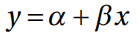
线性函数是一种简单的函数,通常用于从映射层向输出层传递信息。我们在数据变化较小的地方使用线性函数。在深度学习模型中,实践者通常在最后一个隐藏层到输出层之间使用线性函数。在线性函数中,输出总是被限制在一个特定的范围内;因此,它被用于深度学习模型的最后一个隐藏层,或基于线性回归的任务,或在深度学习模型的任务是预测从输入数据集的结果。公式为:
双线性函数
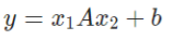
双线性函数是一种用于传递信息的简单函数。它对输入数据应用双线性变换。
import numpy as np
import torch
import torch.nn as nnx1 = torch.randn(100, 10)
x2 = torch.randn(100, 30)
linear = nn.Linear(in_features=10, out_features=5, bias=True)
output_linear = linear(x1)
print("output size:", output_linear.size())
bilinear = nn.Bilinear(in1_features=10, in2_features=30, out_features=5, bias=True)
output_bilinear = bilinear(x1, x2)
print("output size:", output_bilinear.size())
# output size: torch.Size([100, 5])
# output size: torch.Size([100, 5])weight = bilinear.weight.data.cpu().numpy()
bias = bilinear.bias.data.cpu().numpy()
np_x1 = x1.data.cpu().numpy()
np_x2 = x2.data.cpu().numpy()
print(np_x1.shape,weight.shape,np_x2.shape,bias.shape)
# (100, 10) (5, 10, 30) (100, 30) (5,)
y = np.zeros((np_x1.shape[0],weight.shape[0]))
# y.shape (100,5)
for k in range(weight.shape[0]):buff = np.dot(np_x1, weight[k])print(buff.shape)# buff.shape (100, 30)buff = buff * np_x2buff = np.sum(buff,axis=1)print(buff.shape)# buff.shape (100,)y[:,k] = buff
y += bias
dif = y - output_bilinear.data.cpu().numpy()
print(np.mean(np.abs(dif.flatten())))
# 2.2480543702840806e-07
Sigmoid函数
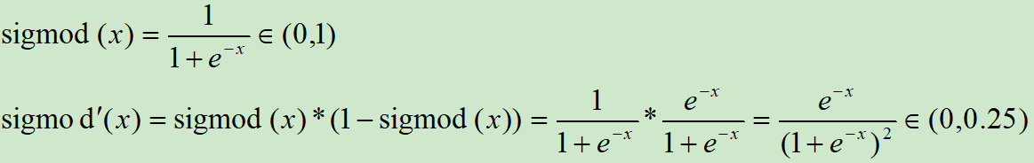
在数据挖掘和分析中,专业人员经常使用sigmoid函数,因为它更容易解释和实现。它是一个非线性函数。当我们将权值从神经网络的输入层传递到隐含层时,我们希望我们的模型能够捕获数据中呈现的所有非线性;因此,建议在神经网络的隐层中使用sigmoid函数。非线性函数有助于泛化数据集。用非线性函数计算函数的梯度比较容易。
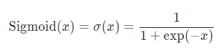
sigmoid函数是一种特殊的非线性激活函数。sigmoid函数的输出总是限制在0和1之内;因此,它主要用于执行基于分类的任务。sigmoid函数的局限性之一是它可能会陷入局部极小值。这样做的好处是,它提供了属于这类的可能性。下面是它的方程。


import torchx = torch.randn(100, 10)
y = torch.randn(100,30)
sig=nn.Sigmoid()
output_sigx = sig(x)
output_sigy = sig(y)
print("Output size:", output_sigx.size())
print("Output size:", output_sigy.size())
print(x[0])
print(output_sigx[0])
# Output size: torch.Size([100, 10])
# Output size: torch.Size([100, 30])
# tensor([ 0.4357, -1.5673, -0.8468,  0.0629, -1.2619, -0.2609, -0.3565,  0.5630, 1.8491,  0.3339])
# tensor([0.6072, 0.1726, 0.3001, 0.5157, 0.2206, 0.4351, 0.4118, 0.6372, 0.8640, 0.5827])class Sigmoid(nn.Module):def __init__(self):super(Sigmoid, self).__init__()def forward(self, x):return 1./(1. + torch.exp(-x))class Sigmoid(nn.Module):def __init__(self):super(Sigmoid, self).__init__()def forward(self, x):return F.sigmoid(x)
双曲正切
双曲正切函数是变换函数的另一种变体。它用于将信息从映射层转换到隐藏层。它通常用于神经网络模型的隐藏层之间。tanh函数的取值范围是-1到+1。公式如下:


import torchx = torch.randn(100, 10)
y = torch.randn(100,30)func = nn.Tanh()
output_x = func(x)
output_y = func(y)
print("Output size:", output_x.size())
print("Output size:", output_y.size())
# Output size: torch.Size([100, 10])
# Output size: torch.Size([100, 30])
print(x[0])
print(output_x[0])
# tensor([-0.2978, -1.0893, -0.3137, -0.5245, -0.1842,  1.6686, -0.7928, -2.2920, -0.8125, -1.9004])
# tensor([-0.2893, -0.7966, -0.3038, -0.4812, -0.1822,  0.9314, -0.6600, -0.9798,-0.6709, -0.9563])class Tanh(nn.Module):def __init__(self):super(Tanh, self).__init__()def forward(self, x):return (torch.exp(x)-torch.exp(-x))/(torch.exp(x)+torch.exp(-x))class Tanh(nn.Module):def __init__(self):super(Tanh, self).__init__()def forward(self, x):return F.tanh(x)
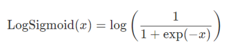
Log Sigmoid 函数
下面的公式解释了用于将输入层映射到隐藏层的log sigmoid传递函数。如果数据不是二进制的,并且它是一个浮点类型,有很多异常值(如输入特征中出现的大数值),那么我们应该使用log sigmoid传递函数。

import torch
x = torch.randn(100, 10)
y = torch.randn(100,30)func = nn.LogSigmoid()
output_x = func(x)
output_y = func(y)
print("Output size:", output_x.size())
print("Output size:", output_y.size())
# Output size: torch.Size([100, 10])
# Output size: torch.Size([100, 30])
print(x[0])
print(output_x[0])
# tensor([-0.6855,  1.1084,  1.0223,  0.8324,  1.0061, -1.4613,  0.7731,  0.0463,0.5831, -0.6826])
# tensor([-1.0935, -0.2852, -0.3073, -0.3612, -0.3116, -1.6699, -0.3795, -0.6702,-0.4435, -1.0916])
ReLU函数
ReLU是另一个激活函数。它用于将信息从输入层传送到输出层。ReLU主要用于卷积神经网络模型。这个激活函数的输出范围是从0到无穷。它主要用于神经网络模型中不同隐藏层之间。


import torch
import torch.nn as nn
x = torch.randn(100, 10)
y = torch.randn(100, 30)func = nn.ReLU()
output_x = func(x)
output_y = func(y)
print("Output size:", output_x.size())
print("Output size:", output_y.size())
# Output size: torch.Size([100, 10])
# Output size: torch.Size([100, 30])
print(x[0])
print(output_x[0])
# tensor([ 0.5594,  0.2387, -1.5372, -0.6874,  1.1714, -0.1458, -1.1784, -0.0802,-0.5905,  2.2499])
# tensor([0.5594, 0.2387, 0.0000, 0.0000, 1.1714, 0.0000, 0.0000, 0.0000, 0.0000,2.2499])def relu(inX):return np.maximum(0,inX)
在神经网络结构中,不同类型的传递函数是可以互换的。它们可以在输入到隐含层、隐含层到输出层等不同阶段使用,以提高模型的精度。
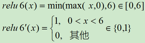
ReLU6函数
Relu在x>0的区域使用x进行线性激活,有可能造成激活后的值太大,影响模型的稳定性,为抵消ReLU激励函数的线性增长部分,可以使用Relu6函数。
ReLU激活函数和导函数分别为:

import torch
import torch.nn as nn
x = torch.randn(100, 10)* 10
y = torch.randn(100, 30) func = nn.ReLU6()
output_x = func(x)
output_y = func(y)
print("Output size:", output_x.size())
print("Output size:", output_y.size())
# Output size: torch.Size([100, 10])
# Output size: torch.Size([100, 30])
print(x[0])
print(output_x[0])
# tensor([  8.1576,  11.7024,  -3.9226,  -2.6406,  11.0565, -16.3319,   7.0528, 0.8866,   0.6748,  -1.0607])
# tensor([6.0000, 6.0000, 0.0000, 0.0000, 6.0000, 0.0000, 6.0000, 0.8866, 0.6748, 0.0000])
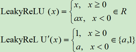
Leaky ReLU函数
在标准的神经网络模型中,死亡梯度问题是常见的。为了避免这个问题,应用了leaky ReLU。Leaky ReLU允许一个小的非零梯度。
LeakyReLU函数与倒数分别为:

import torch
import torch.nn as nn
x = torch.randn(100, 10)
y = torch.randn(100, 30)func = nn.LeakyReLU()
output_x = func(x)
output_y = func(y)
print("Output size:", output_x.size())
print("Output size:", output_y.size())
# Output size: torch.Size([100, 10])
# Output size: torch.Size([100, 30])
print(x[0])
print(output_x[0])
# tensor([ 1.0718, -0.3105, -0.2773,  1.8701,  0.2646, -0.2166,  1.1425,  1.1959,-2.7848, -0.2138])
# tensor([ 1.0718, -0.0031, -0.0028,  1.8701,  0.2646, -0.0022,  1.1425,  1.1959, -0.0278, -0.0021])
PRELU函数
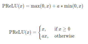
这里a是一个可学习的参数。当不带参数调用时,nn.PReLU()在所有输入通道中使用单个参数a。如果使用nn.PReLU(nChannels)调用,则每个输入通道使用一个单独的a。n_channels表示第二维度数量。

import torch
import torch.nn as nn
x = torch.randn(100, 10)
# torch.nn.PReLU(num_parameters=1, init=0.25, device=None, dtype=None)
# num_parameters表示要学习的a的数量。尽管它接受一个int作为输入,但只有两个值是合法的:1,或者输入处的通道数量。默认值:1
# init:a的初始值,默认是0.25
func = nn.PReLU(10)
y = func(x)
print(x[0])
print(y[0])
# tensor([-0.5982, -0.5509, -0.7107, -0.4316, -0.5107,  0.4100, -1.3367,  1.5206, -2.4008, -1.1881])
# tensor([-0.1495, -0.1377, -0.1777, -0.1079, -0.1277,  0.4100, -0.3342,  1.5206, -0.6002, -0.2970], grad_fn=<SelectBackward>)
RReLU函数
在RReLU中,负值的斜率在训练中是随机的,在之后的测试中就变成了固定的了。RReLU的亮点在于,在训练环节中,a是从一个均匀的分布U(I,u)中随机抽取的数值。
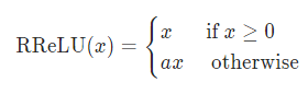
RReLU中的a是一个在一个给定的范围内随机抽取的值,这个值在测试环节就会固定下来。

import torch
import torch.nn as nn
x = torch.randn(100, 10)
# torch.nn.RReLU(lower=0.125, upper=0.3333333333333333, inplace=False)
func = nn.RReLU(0.1, 0.3)
y = func(x)
print(x[0])
print(y[0])
# tensor([-0.4467,  0.3433,  0.0522,  0.5509,  1.7010, -0.1909,  0.6914, -0.6053, 0.5511, -1.9335])
# tensor([-0.0514,  0.3433,  0.0522,  0.5509,  1.7010, -0.0270,  0.6914, -0.1125, 0.5511, -0.5593])
ELU函数
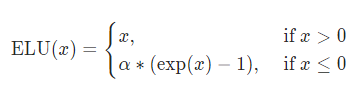
α \alpha α:默认为1.0
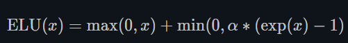
其中α是一个可调整的参数,它控制着ELU负值部分在何时饱和。右侧线性部分使得ELU能够缓解梯度消失,而左侧软饱能够让ELU对输入变化或噪声更鲁棒。ELU的输出均值接近于零,所以收敛速度更快.

import torch
import torch.nn as nn
x = torch.randn(100, 10)
# torch.nn.SELU(inplace=False)
func = nn.ELU()
y = func(x)
print(x[0])
print(y[0])
# tensor([-0.6763,  0.6669, -2.0544, -1.8889, -0.3581,  0.0884, -1.3734,  0.9181,0.4205,  0.1281])
# tensor([-0.4915,  0.6669, -0.8718, -0.8488, -0.3010,  0.0884, -0.7467,  0.9181,0.4205,  0.1281])import torch
import torch.nn as nn
import torch.nn.functional as F
import matplotlib.pyplot as pltclass ELU(nn.Module):def __init__(self):super().__init__()def forward(self,x):x = F.elu(x)return xclass ELU(nn.Module):def __init__(self, alpha=1.0):super(ELU, self).__init__()self.alpha=alphadef forward(self, x):temp1 = F.relu(x)temp2 = self.alpha * (-1*F.relu(1-torch.exp(x)))return temp1 + temp2
x = torch.linspace(-10, 10, 1000).unsqueeze(0)func = nn.ELU()
func2 = ELU()y1 = func(x)
y2 = func2(x)plt.plot(x.detach().numpy()[0],y1.detach().numpy()[0],label="PyTorch")
plt.plot(x.detach().numpy()[0],y2.detach().numpy()[0],label="myELU")
plt.legend()
plt.grid()
plt.show()

CELU函数
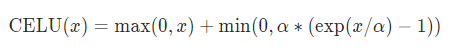
α \alpha α:默认为1.0

import torch
import torch.nn as nn
x = torch.randn(100, 10)
# torch.nn.SELU(inplace=False)
func = nn.CELU()
y = func(x)
print(x[0])
print(y[0])
# tensor([-1.1315, -0.3425,  0.7596, -1.8625, -0.8638,  0.2654,  0.9773, -0.5946, 0.1348, -0.7941])
# tensor([-0.6775, -0.2900,  0.7596, -0.8447, -0.5785,  0.2654,  0.9773, -0.4482, 0.1348, -0.5480])import torch
import torch.nn as nn
import torch.nn.functional as F
from matplotlib import pyplot as plt
class CELU(nn.Module):def __init__(self, alpha=1.0):super(CELU, self).__init__()self.alpha=alphadef forward(self, x):temp1 = F.relu(x)# temp2 = self.alpha * (F.elu(-1*F.relu(-1.*x/self.alpha)))temp2 = self.alpha * (-1*F.relu(1-torch.exp(x/self.alpha)))return temp1 + temp2x = torch.linspace(-10, 10, 1000).unsqueeze(0)func = nn.CELU()
func2 = CELU()y1 = func(x)
y2 = func2(x)plt.plot(x.detach().numpy()[0],y1.detach().numpy()[0],label="PyTorch")
plt.plot(x.detach().numpy()[0],y2.detach().numpy()[0],label="myCELU")
plt.legend()
plt.grid()
plt.show()

SELU函数
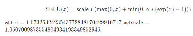
此处的scale就是下方的 λ \lambda λ


当使用kaiming_normal或kaiming_normal_进行初始化时,为了得到自归一化的神经网络,应该使用nonlinearity='linear’而不是nonlinearity=‘selu’。
经过该激活函数后使得样本分布自动归一化到0均值和单位方差(自归一化,保证训练过程中梯度不会爆炸或消失,效果比Batch Normalization 要好)
关键在于这个 λ \lambda λ是大于1的,在方差过小的的时候可以让它增大,同时防止了梯度消失。
import torch
import torch.nn as nn
import torch.nn.functional as F
from matplotlib import pyplot as plt
class SELU(nn.Module):def __init__(self):super(SELU, self).__init__()self.alpha = 1.6732632423543772848170429916717self.scale = 1.0507009873554804934193349852946def forward(self, x):temp1 = self.scale * F.relu(x)# temp2 = self.scale * self.alpha * (F.elu(-1*F.relu(-1*x)))temp2 = self.scale * self.alpha * (-1*F.relu(1-torch.exp(x)))return temp1 + temp2x = torch.linspace(-10, 10, 1000).unsqueeze(0)func2 = nn.SELU()
func = SELU()y1 = func(x)
y2 = func2(x)plt.plot(x.detach().numpy()[0],y1.detach().numpy()[0],label="mySELU")
plt.plot(x.detach().numpy()[0],y2.detach().numpy()[0],label="PyTorch")
plt.legend()
plt.grid()
plt.show()

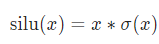
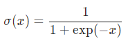
SiLU函数(swish)

import torch
import torch.nn as nn
import torch.nn.functional as F
from matplotlib import pyplot as plt
class SiLU(nn.Module):def __init__(self):super(SiLU, self).__init__()def forward(self, x):return x * F.sigmoid(x)x = torch.linspace(-10, 10, 1000).unsqueeze(0)
# torch.nn.SELU(inplace=False)
func = nn.SiLU()
func2 = SiLU()y1 = func(x)
y2 = func2(x)plt.plot(x.detach().numpy()[0],y1.detach().numpy()[0],label="mySiLU")
plt.plot(x.detach().numpy()[0],y2.detach().numpy()[0],label="PyTorch")
plt.legend()
plt.grid()
plt.show()

Hardswish函数
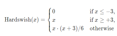
数值稳定性好,计算速度快等优点。
import torch
import torch.nn as nn
import torch.nn.functional as F
from matplotlib import pyplot as plt'''Hard Swish Module'''
class HardSwish(nn.Module):def __init__(self, inplace=False):super(HardSwish, self).__init__()self.act = nn.ReLU6(inplace)'''forward'''def forward(self, x):return x * self.act(x + 3) / 6x = torch.arange(-50, 50).unsqueeze(0)
func = HardSwish()
output_x = func(x)
plt.plot(x.detach().numpy()[0],output_x.detach().numpy()[0],label="HardSwish")
plt.legend()
plt.grid()
plt.show()

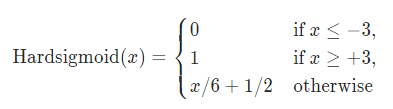
HardSigmod函数
import torch
import torch.nn as nn'''Hard Sigmoid Module'''
class HardSigmoid(nn.Module):def __init__(self, bias=1.0, divisor=2.0, min_value=0.0, max_value=1.0):super(HardSigmoid, self).__init__()assert divisor != 0, 'divisor is not allowed to be equal to zero'self.bias = biasself.divisor = divisorself.min_value = min_valueself.max_value = max_value'''forward'''def forward(self, x):x = (x + self.bias) / self.divisorreturn x.clamp_(self.min_value, self.max_value)
x = torch.linspace(-5, 5, 100).unsqueeze(0)
func = HardSigmoid()
output_x = func(x)
plt.plot(x.detach().numpy()[0],output_x.detach().numpy()[0],label="HardSigmoid")
plt.legend()
plt.grid()
plt.show()

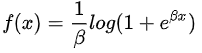
Softplus函数
SoftPlus是一个平滑的近似于ReLU函数,可以用来约束输出总是正的。

import numpy as np
x = np.linspace(-10, 10, 100)
y1 = np.log(1 + np.exp(x))
y2 = np.maximum(0, x)
plt.plot(x,y1,label="softplus")
plt.plot(x,y2,label="relu")
plt.legend()
plt.show()import torch
import torch.nn as nn
x = torch.randn(100, 10)
y = torch.randn(100, 30)
# torch.nn.Softplus(beta=1, threshold=20)
func = nn.Softplus()
output_x = func(x)
output_y = func(y)
print("Output size:", output_x.size())
print("Output size:", output_y.size())
# Output size: torch.Size([100, 10])
# Output size: torch.Size([100, 30])
print(x[0])
print(output_x[0])
# tensor([ 2.6387,  0.6161, -0.0684, -0.3626,  2.2955, -0.1481, -0.1116,  0.1727, 0.2522,  0.6943])
# tensor([2.7077, 1.0479, 0.6595, 0.5282, 2.3915, 0.6218, 0.6389, 0.7832, 0.8272, 1.0994])class Softplus(nn.Module):def __init__(self, beta=1):super(Softplus, self).__init__()self.beta = betaassert beta !=0, "beta should not be equal to 0"def forward(self, x):return 1./beta * torch.log(1 + torch.exp(beta * x))
class Softplus(nn.Module):def __init__(self, beta=1.):super(Softplus, self).__init__()self.beta = betaassert beta !=0, "beta should not be equal to 0"def forward(self, x):return F.softplus(x, beta)
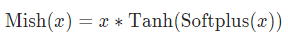
Mish函数
# -*- coding: utf-8 -*-
import torch
import torch.nn as nn
import torch.nn.functional as F
from matplotlib import pyplot as pltclass Mish(nn.Module):def __init__(self):super().__init__()print("Mish activation loaded...")def forward(self,x):x = x * (torch.tanh(F.softplus(x)))return xmish = Mish()
x = torch.linspace(-10,10,1000)
y1 = mish(x)
# func = nn.Mish()  # PyTorch1.9才有Mish激活函数
# y2 = func(x)plt.plot(x,y1,label="myMish")
# plt.plot(x,y2,label="PyTorch")
plt.legend()
plt.show()
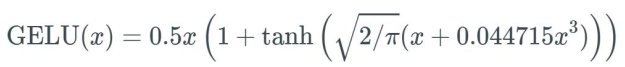
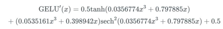
GELU函数
高斯误差线性单元激活函数在最近的 Transformer 模型(谷歌的 BERT 和 OpenAI 的 GPT-2)中得到了应用。
激活函数:

导数:

import torch.nn as nn
import torch
import matplotlib.pyplot as plt
import numpy as npclass GELU(nn.Module):def __init__(self, beta=1):super(GELU, self).__init__()def forward(self, x):return F.gelu(x)class GELU(nn.Module):def __init__(self, beta=1):super(GELU, self).__init__()def forward(self, x):x_= np.sqrt(2./np.pi) * (x+0.044715 * x * x * x)return 0.5 * x * (1 + (torch.exp(x_) - torch.exp(-x_))/(torch.exp(x_) + torch.exp(-x_)))x = torch.linspace(-10, 10, 1000).unsqueeze(0)
# torch.nn.SELU(inplace=False)
func2 = nn.GELU()
func = GELU()y1 = func(x)
y2 = func2(x)plt.plot(x.detach().numpy()[0],y1.detach().numpy()[0],label="myGELU")
plt.plot(x.detach().numpy()[0],y2.detach().numpy()[0],label="PyTorch")
plt.legend()
plt.grid()
plt.show()

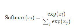
softmax函数
Softmax 函数对 n 维输入 Tensor 进行重新缩放,以便 n 维输出 Tensor 的值位于 [0,1] 范围内并且总和为 1。当输入张量是一个稀疏张量时,未指定的值被视为负无穷。
import torch
import torch.nn as nn
import torch.nn.functional as F
from matplotlib import pyplot as pltclass Softmax(nn.Module):def __init__(self, dim=1):super().__init__()self.dim= dimprint("Softmax activation loaded...")def forward(self,X):X_exp = X.exp()partion = X_exp.sum(dim=self.dim, keepdim=True)  # 沿着列方向求和,即对每一行求和return X_exp/partion  # 广播机制,partion被扩展成与X_exp同shape的,对应位置元素做除法func= Softmax()
x = torch.linspace(-20,20,1000).unsqueeze(0)
y1 = func(x)func2 = nn.Softmax(dim=1)
y2 = func2(x)plt.plot(x.detach().numpy()[0],y1.detach().numpy()[0],label="mySoftmax")
plt.plot(x.detach().numpy()[0],y2.detach().numpy()[0],label="PyTorch")
plt.legend()
plt.show()

这个模块不直接与NLLLoss一起工作,它期望在Softmax和NLLLoss之间添加计算log的操作。使用LogSoftmax代替(它更快并且有更好的数值属性)。
总结
本章讨论了各种激活函数以及在各种情况下激活函数的使用。选择最佳激活函数的方法是精度驱动的;在模型中,应该始终使用能给出最佳结果的激活函数。
参考资料
https://blog.csdn.net/qq_20909377/article/details/79133981
https://blog.csdn.net/weixin_42528089/article/details/84865069
https://www.cnblogs.com/wqbin/p/11099612.html
https://blog.csdn.net/tototuzuoquan/article/details/113791252
https://pytorch.org/
https://blog.csdn.net/qq_24819773/article/details/104439170