RRT 算法研究
参考
机器人路径规划、轨迹优化课程-第五讲-RRT算法原理和代码讲解
机器人路径规划之RRT算法(附C++源码)
RRT算法(快速拓展随机树)的Python实现
《基于改进RRT算法的路径规划研究》
《面向室内复杂场景的移动机器人快速路径规划算法研究》
理论基础
RRT(Rapidly-Exploring Random Trees)算法是一种用于路径规划的随机采样算法,特别适用于高维空间中的运动规划问题。它通过在配置空间中随机采样,并使用启发式规则和随机树的构建来搜索可行路径
下面是RRT算法的一般步骤:
- 初始化树:创建一个只包含起始节点的树
- 随机采样:从配置空间中随机采样一个节点
- 最近邻节点选择:在树中找到距离随机采样节点最近的节点
- 扩展节点:从最近邻节点沿着一定步长向随机采样节点方向扩展,得到一个新的节点
- 碰撞检测:检查新节点与障碍物之间是否存在碰撞
- 添加节点:如果新节点通过碰撞检测,将其添加到树中,并将其与最近邻节点连接
- 判断终止条件:如果新节点接近目标节点(达到一定距离范围内),或者达到最大迭代次数,算法结束
- 重复上述步骤2到步骤7,直到满足终止条件
- 路径提取:从终止节点回溯到起始节点,构建可行路径
RRT算法的优点是能够在高维配置空间中搜索到可行路径,并且算法的实现相对简单。然而,它并不能保证找到全局最优解,因为它是基于随机采样的方法,路径的质量取决于采样的随机性和树的生长方式
伪代码如下

算法流程图如下

Python 实现
import matplotlib.pyplot as plt
import random
import math
import copyshow_animation = Trueclass Node(object):"""RRT Node"""def __init__(self, x, y):self.x = xself.y = yself.parent = Noneclass RRT(object):"""Class for RRT Planning"""def __init__(self, start, goal, obstacle_list, rand_area):"""Setting Parameterstart:Start Position [x,y]goal:Goal Position [x,y]obstacleList:obstacle Positions [[x,y,size],...]randArea:random sampling Area [min,max]"""self.start = Node(start[0], start[1])self.end = Node(goal[0], goal[1])self.min_rand = rand_area[0]self.max_rand = rand_area[1]self.expandDis = 1.0self.goalSampleRate = 0.05self.maxIter = 500self.obstacleList = obstacle_listself.nodeList = [self.start]def random_node(self):""":return:"""node_x = random.uniform(self.min_rand, self.max_rand)node_y = random.uniform(self.min_rand, self.max_rand)node = [node_x, node_y]return node@staticmethoddef get_nearest_list_index(node_list, rnd):""":param node_list::param rnd::return:"""d_list = [(node.x - rnd[0]) ** 2 + (node.y - rnd[1]) ** 2 for node in node_list]min_index = d_list.index(min(d_list))return min_index@staticmethoddef collision_check(new_node, obstacle_list):a = 1for (ox, oy, size) in obstacle_list:dx = ox - new_node.xdy = oy - new_node.yd = math.sqrt(dx * dx + dy * dy)if d <= size:a = 0  # collisionreturn a  # safedef planning(self):"""Path planninganimation: flag for animation on or off"""while True:# Random Samplingif random.random() > self.goalSampleRate:rnd = self.random_node()else:rnd = [self.end.x, self.end.y]# Find nearest nodemin_index = self.get_nearest_list_index(self.nodeList, rnd)# print(min_index)# expand treenearest_node = self.nodeList[min_index]theta = math.atan2(rnd[1] - nearest_node.y, rnd[0] - nearest_node.x)new_node = copy.deepcopy(nearest_node)new_node.x += self.expandDis * math.cos(theta)new_node.y += self.expandDis * math.sin(theta)new_node.parent = min_indexif not self.collision_check(new_node, self.obstacleList):continueself.nodeList.append(new_node)# check goaldx = new_node.x - self.end.xdy = new_node.y - self.end.yd = math.sqrt(dx * dx + dy * dy)if d <= self.expandDis:print("Goal!!")breakif True:self.draw_graph(rnd)path = [[self.end.x, self.end.y]]last_index = len(self.nodeList) - 1while self.nodeList[last_index].parent is not None:node = self.nodeList[last_index]path.append([node.x, node.y])last_index = node.parentpath.append([self.start.x, self.start.y])path = path[::-1]return pathdef draw_graph(self, rnd=None):"""Draw Graph"""plt.clf()if rnd is not None:plt.plot(rnd[0], rnd[1], "^g")for node in self.nodeList:if node.parent is not None:plt.plot([node.x, self.nodeList[node.parent].x], [node.y, self.nodeList[node.parent].y], "-g")for (ox, oy, size) in self.obstacleList:plt.plot(ox, oy, "sk", ms=10*size)plt.plot(self.start.x, self.start.y, "^r")plt.plot(self.end.x, self.end.y, "^b")plt.axis([self.min_rand, self.max_rand, self.min_rand, self.max_rand])plt.grid(True)plt.pause(0.01)def draw_static(self, path):""":return:"""plt.clf()for node in self.nodeList:if node.parent is not None:plt.plot([node.x, self.nodeList[node.parent].x], [node.y, self.nodeList[node.parent].y], "-g")for (ox, oy, size) in self.obstacleList:plt.plot(ox, oy, "sk", ms=10*size)plt.plot(self.start.x, self.start.y, "^r")plt.plot(self.end.x, self.end.y, "^b")plt.axis([self.min_rand, self.max_rand, self.min_rand, self.max_rand])plt.plot([data[0] for data in path], [data[1] for data in path], '-r')plt.grid(True)plt.show()def main():print("start RRT path planning")obstacle_list = [(5, 1, 1),(3, 6, 2),(3, 8, 2),(1, 1, 2),(3, 5, 2),(9, 5, 2)]# Set Initial parametersrrt = RRT(start=[0, 0], goal=[8, 9], rand_area=[-2, 10], obstacle_list=obstacle_list)path = rrt.planning()print(path)# Draw final pathif show_animation:plt.close()rrt.draw_static(path)if __name__ == '__main__':main()
运行输出
start RRT path planning
Goal!!
[[0, 0], [-0.14022396397750916, -0.9901198108948402], [0.8585235952215351, -1.0401529298656953], [1.8548573532880313, -0.9546015269719231], [2.8137704966221295, -1.2383013393460578], [3.6579610280508703, -0.7022581072779154], [4.256013896993427, 0.09919854529262528], [3.467716060357506, 0.7144923944046785], [3.559533505502979, 1.7102682510948064], [3.3748555983072857, 2.693067350908099], [4.228916724760976, 3.213240007129717], [4.922837650396268, 3.933291219867713], [5.907104096947173, 4.109981803074782], [6.30057446621359, 5.029319101627033], [6.694044835480005, 5.948656400179284], [7.536173615685667, 6.487932876162915], [6.987665020486496, 7.324077792426018], [7.504705318909289, 8.180038848670325], [8, 9]]

与 RRT 算法对应的逻辑主要在 planning 函数中
def planning(self):"""Path planninganimation: flag for animation on or off"""while True:# Random Samplingif random.random() > self.goalSampleRate:rnd = self.random_node()else:rnd = [self.end.x, self.end.y]# Find nearest nodemin_index = self.get_nearest_list_index(self.nodeList, rnd)# print(min_index)# expand treenearest_node = self.nodeList[min_index]theta = math.atan2(rnd[1] - nearest_node.y, rnd[0] - nearest_node.x)new_node = copy.deepcopy(nearest_node)new_node.x += self.expandDis * math.cos(theta)new_node.y += self.expandDis * math.sin(theta)new_node.parent = min_indexif not self.collision_check(new_node, self.obstacleList):continueself.nodeList.append(new_node)# check goaldx = new_node.x - self.end.xdy = new_node.y - self.end.yd = math.sqrt(dx * dx + dy * dy)if d <= self.expandDis:print("Goal!!")breakif True:self.draw_graph(rnd)path = [[self.end.x, self.end.y]]last_index = len(self.nodeList) - 1while self.nodeList[last_index].parent is not None:node = self.nodeList[last_index]path.append([node.x, node.y])last_index = node.parentpath.append([self.start.x, self.start.y])path = path[::-1]return path
1、随机采样路径点
# Random Samplingif random.random() > self.goalSampleRate:rnd = self.random_node()else:rnd = [self.end.x, self.end.y]
2、获取离采样点最近的已添加的路径点
# Find nearest nodemin_index = self.get_nearest_list_index(self.nodeList, rnd)# print(min_index)# expand treenearest_node = self.nodeList[min_index]
3、生成新的路径点并进行膨胀检测,未发生碰撞则加入路径点集中
new_node = copy.deepcopy(nearest_node)new_node.x += self.expandDis * math.cos(theta)new_node.y += self.expandDis * math.sin(theta)new_node.parent = min_indexif not self.collision_check(new_node, self.obstacleList):continueself.nodeList.append(new_node)
4、检查终点是否在以新节点为圆心,步长为半径的圆内,在的话则退出循环
# check goaldx = new_node.x - self.end.xdy = new_node.y - self.end.yd = math.sqrt(dx * dx + dy * dy)if d <= self.expandDis:print("Goal!!")breakif True:self.draw_graph(rnd)
5、通过节点中的 parent 属性回溯出规划的路径
path = [[self.end.x, self.end.y]]last_index = len(self.nodeList) - 1while self.nodeList[last_index].parent is not None:node = self.nodeList[last_index]path.append([node.x, node.y])last_index = node.parentpath.append([self.start.x, self.start.y])path = path[::-1]
C++ 实现
https://github.com/kushuaiming/planning_algorithm/tree/master
头文件如下,rrt.h
#ifndef RRT_H_
#define RRT_H_#include <cmath>
#include <iostream>
#include <opencv2/opencv.hpp>
#include <random>
#include <vector>struct Point {Point(double x, double y) : x(x), y(y) {}double x = 0.0;double y = 0.0;
};class Node {public:Node(double x, double y) : point_(x, y), parent_(nullptr), cost_(0.0) {}const Point& point() const { return point_; }void set_parent(Node* parent) { parent_ = parent; }Node* parent() { return parent_; }private:Point point_;std::vector<double> path_x_;std::vector<double> path_y_;Node* parent_ = nullptr;double cost_ = 0.0;
};class RRT {public:RRT(Node* start_node, Node* goal_node,const std::vector<std::vector<double>>& obstacle_list,double step_size = 1.0, int goal_sample_rate = 5): start_node_(start_node),goal_node_(goal_node),obstacle_list_(obstacle_list),step_size_(step_size),goal_sample_rate_(goal_sample_rate),goal_gen_(goal_rd_()),goal_dis_(std::uniform_int_distribution<int>(0, 100)),area_gen_(area_rd_()),area_dis_(std::uniform_real_distribution<double>(0, 15)) {}Node* GetNearestNode(const std::vector<double>& random_position);bool CollisionCheck(Node*);std::vector<Node*> Planning();private:Node* start_node_;Node* goal_node_;std::vector<std::vector<double>> obstacle_list_;std::vector<Node*> node_list_;double step_size_;int goal_sample_rate_;std::random_device goal_rd_;std::mt19937 goal_gen_;std::uniform_int_distribution<int> goal_dis_;std::random_device area_rd_;std::mt19937 area_gen_;std::uniform_real_distribution<double> area_dis_;
};#endif

与 RRT 算法对应的逻辑主要也是在 Planning 函数中,只是语法不同,不再赘述
std::vector<Node*> RRT::Planning() {cv::namedWindow("RRT");int count = 0;constexpr int kImageSize = 15;constexpr int kImageResolution = 50;cv::Mat background(kImageSize * kImageResolution,kImageSize * kImageResolution, CV_8UC3,cv::Scalar(255, 255, 255));circle(background,cv::Point(start_node_->point().x * kImageResolution,start_node_->point().y * kImageResolution),20, cv::Scalar(0, 0, 255), -1);circle(background,cv::Point(goal_node_->point().x * kImageResolution,goal_node_->point().y * kImageResolution),20, cv::Scalar(255, 0, 0), -1);for (auto item : obstacle_list_) {circle(background,cv::Point(item[0] * kImageResolution, item[1] * kImageResolution),item[2] * kImageResolution, cv::Scalar(0, 0, 0), -1);}node_list_.push_back(start_node_);while (1) {std::vector<double> random_position;if (goal_dis_(goal_gen_) > goal_sample_rate_) {double randX = area_dis_(goal_gen_);double randY = area_dis_(goal_gen_);random_position.push_back(randX);random_position.push_back(randY);} else {random_position.push_back(goal_node_->point().x);random_position.push_back(goal_node_->point().y);}Node* nearestNode = GetNearestNode(random_position);double theta = atan2(random_position[1] - nearestNode->point().y,random_position[0] - nearestNode->point().x);Node* newNode = new Node(nearestNode->point().x + step_size_ * cos(theta),nearestNode->point().y + step_size_ * sin(theta));newNode->set_parent(nearestNode);if (!CollisionCheck(newNode)) continue;node_list_.push_back(newNode);line(background,cv::Point(static_cast<int>(newNode->point().x * kImageResolution),static_cast<int>(newNode->point().y * kImageResolution)),cv::Point(static_cast<int>(nearestNode->point().x * kImageResolution),static_cast<int>(nearestNode->point().y * kImageResolution)),cv::Scalar(0, 255, 0), 10);count++;imshow("RRT", background);cv::waitKey(5);if (sqrt(pow(newNode->point().x - goal_node_->point().x, 2) +pow(newNode->point().y - goal_node_->point().y, 2)) <=step_size_) {std::cout << "The path has been found!" << std::endl;break;}}std::vector<Node*> path;path.push_back(goal_node_);Node* tmp_node = node_list_.back();while (tmp_node->parent() != nullptr) {line(background,cv::Point(static_cast<int>(tmp_node->point().x * kImageResolution),static_cast<int>(tmp_node->point().y * kImageResolution)),cv::Point(static_cast<int>(tmp_node->parent()->point().x * kImageResolution),static_cast<int>(tmp_node->parent()->point().y * kImageResolution)),cv::Scalar(255, 0, 255), 10);path.push_back(tmp_node);tmp_node = tmp_node->parent();}imshow("RRT", background);cv::waitKey(0);path.push_back(start_node_);return path;
}
代码注意点
上面的 Python 实现和 C++ 实现中都有两个需要注意的地方
1、在迭代采用的过程中均为设置最大迭代次数,如果终点就是障碍物可能会导致死循环
2、代码实现的 RRT 算法并不是纯粹的原始的 RRT 算法,而是基于概率的 RRT 算法
为了加快随机树收敛到目标位置的速度,基于概率的RRT算法在随机树的扩展的步骤中引入一个概率p,根据概率 p 的值来选择树的生长方向是随机生长(Node_rand)还是朝向目标位置(Node_goal)生长。引入向目标生长的机制可以加速路径搜索的收敛速度
基于概率的 RRT 算法也可以叫做 Goal-Bias RRT算法,该算法将目标节点作为采样点出现,并且算法中还可以控制目标点出现的概率
RRT算法相较于其他路径规划算法如栅格法,A* ,D*算法等,一大特点在于对空间的随机搜索,这样的搜索尤其给高维空间的路径规划带来了巨大优势,但是这样的搜索同样带给RRT 算法一大缺点:算法的运算效率不高。随机树搜索漫无目的,在整个度量空间生成随机点,依据随机点进行随机树扩展,直到恰好有节点扩展到目标附近才结束搜索,生成最终路径。这样的方法虽然能够保证对整个度量空间有效的探索,使得路径解的可能性大大增加,但是在得到路径解之前,随机树经常扩展到一些离目标很远的地方,也就是扩展到离我们期待的目标区域较远的“无用区域”。为了高算法的效率,我们希望随机树的搜索并不是完全漫无目的的,在通常的路径规划任务中,快速到达目标是我们的追求,因此我们希望随机树尽可能向着目标方向搜索,以加快搜索速度
具体的操作方法是:人为地引导随机点的生成,在产生随机点 Node_rand 时,以一定的概率选取目标点(Node_goal)作为循环中的随机点 Node_rand,即 Node_rand = Node_goal
Node_rand 在随机树扩展中相当于给定了一个扩展方向,以一定的概率将目标点作为随机点,等价于驱使随机树向目标方向扩展,算法流程如下

为了保持随机树对未知空间的扩展能力,概率通常不宜选择的过大(通常0.05-0.1)。这种目标偏好的随机树扩展一个显著的缺点是,容易陷入局部搜索无法跳出,尤其是障碍物遮挡目标时。随着目标偏好的程度加大,跳出局部搜索困难越大。因此目标偏好概率的选取要折衷算法效率和RRT扩展能力
这在代码中体现在如下部分
std::vector<double> random_position;if (goal_dis_(goal_gen_) > goal_sample_rate_) {double randX = area_dis_(goal_gen_);double randY = area_dis_(goal_gen_);random_position.push_back(randX);random_position.push_back(randY);} else {random_position.push_back(goal_node_->point().x);random_position.push_back(goal_node_->point().y);}
# Random Samplingif random.random() > self.goalSampleRate:rnd = self.random_node()else:rnd = [self.end.x, self.end.y]
RRT 的改进及变体
由于传统RRT算法规划出的路径是非最优的,为进一步提升规划路径质量,在2011年由Frazzoli提出RRT*算法*。此算法以提升规划路径的相对最优性为目标。传统RRT算法在寻找到初始路径后即结束算法运行,RRT算法继续其迭代过程,通过不断地采样,寻找到相较于原始路径距离更短的路径
其中两种算法最大的区别在于 RRT* 算法可以对父节点进行重新选择,改变原始路径,使规划路径渐进最优
从1998年出现RRT算法,经过近几十年的发展,RRT算法主要可分为两大类。第一类是在传统RRT算法的基础上进行算法改进,第二类是在RRT*算法的基础上进行改进
针对第一类算法,其主要的目标在于以最快的速度、最短的时间内寻找到一条初始路径,但是受限于RRT算法本身的概率完备性和非最优性,使得所规划的路径的质量不是很高,但是其占用计算量小,规划速度快,尤其是在高维的环境中,相较于其他两种全局规划算法,效率有很大的提升。因此,对于RRT算法的优化也来自于对算法概率完备性、非最优性、路线光滑程度等方面的优化。下表汇总了近些年来对RRT算法的一些代表性改进算法:

针对第二类算法,RRT主要的优势在于,其改进了传统RRT算法的规划路径的非最优性。在保证迭代次数的情况下,RRT算法规划出的路径是渐进趋向于最优路径,但是在时间效率方面,其需要消耗更多的时间通过多次迭代来优化当前路径
此外,其计算量相较于传统RRT算法也会有明显的提升。因此,在路径规划选择算法时,重要的指标选取也指明了相应的规划算法。RRT算法,通过单一算法可以使最后规划的路径的质量远远高于传统RRT算法。基于此,学者们在保证RRT算法的优势同时提出了众多的改进算法。下表汇总了近些年来对RRT算法的一些代表性改进算法: