一、 LSTM网络原理
- 要点介绍
(1)LSTM网络用来处理带“序列”(sequence)性质的数据,比如时间序列的数据,像每天的股价走势情况,机械振动信号的时域波形,以及类似于自然语言这种本身带有顺序性质的由有序单词组合的数据。
(2)LSTM本身不是一个独立存在的网络结构,只是整个神经网络的一部分,即由LSTM结构取代原始网络中的隐层单元部分。
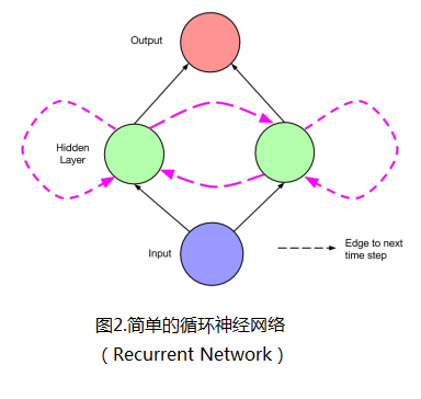
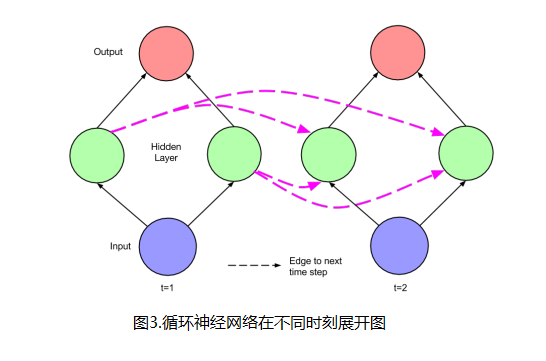
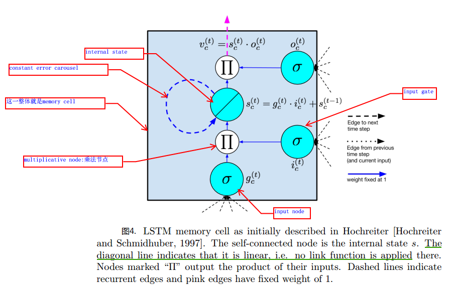
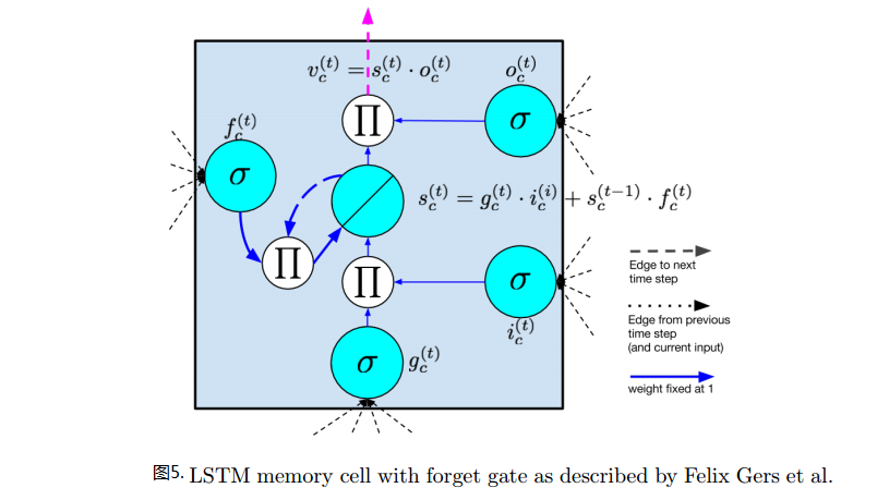
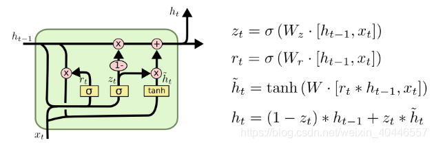
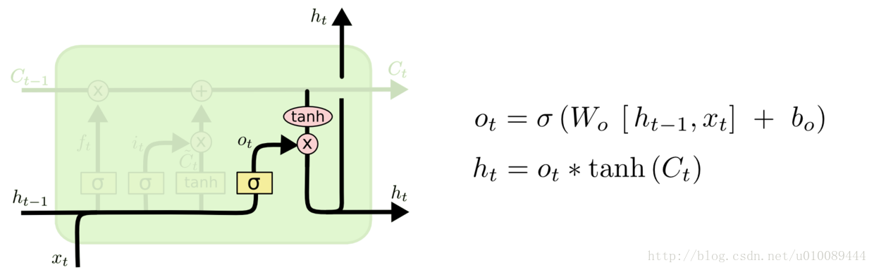
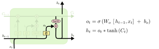
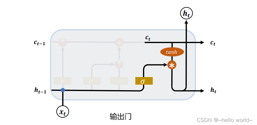
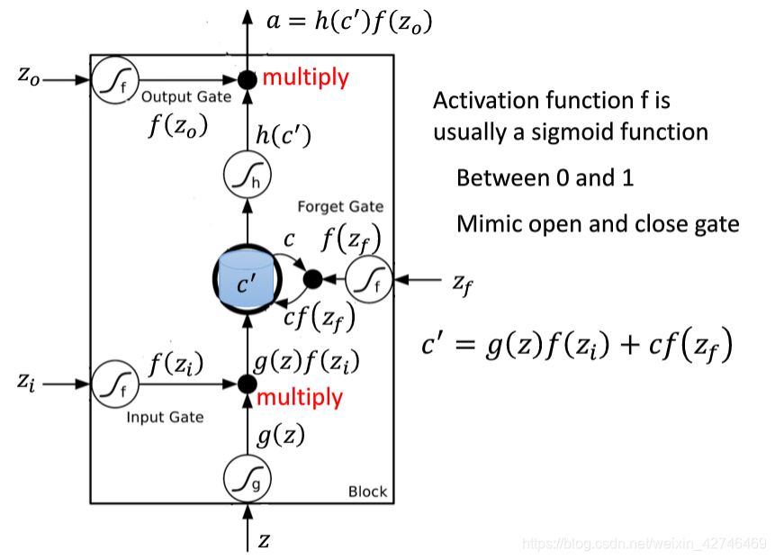
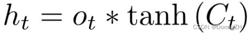
(3)LSTM网络具有“记忆性”。其原因在于不同“时间点”之间的网络存在连接,而不是单个时间点处的网络存在前馈或者反馈。如下图2中的LSTM单元(隐层单元)所示。图3是不同时刻情况下的网络展开图。图中虚线连接代表时刻,“本身的网络”结构连接用实线表示。
2.LSTM单元结构图
图4,5是现在比较常用的LSTM单元结构示意图:
其主要结构成分包含如下:
(1)输入节点input node:接受上一时刻隐层单元的输出及当前时刻是样本输入;
(2)输入门input gate:可以看到输入门会和输入节点的值相乘,组成LSTM中internal state单元值的一部分,当门的输出为1时,输入节点的激活值全部流向internal state,当门的输出为0时,输入节点的值对internal state没有影响。
(3)内部状态internal state。
(4)遗忘门forget gate:用于刷新internal state的状态,控制internal state的上一状态对当前状态的影响。
各节点及门与隐藏单元输出的关系参见图4,图5所示。
二、代码示例
1.示例介绍
主要以今年参加的“2016年阿里流行音乐趋势预测”为例。
时间过得很快,今天已是第二赛季的最后一天了,我从5.18开始接触赛题,到6.14上午10点第一赛季截止,这一期间,由于是线下赛,可以用到各种模型,而自已又是做深度学习(deep learning)方向的研究,所以选择了基于LSTM的循环神经网络模型,结果也很幸运,进入到了第二赛季。开始接触深度学习也有大半年了,能够将自已所学用到这次真正的实际生活应用中,结果也还可以,自已感觉很欣慰。突然意识到,自已学习生涯这么多年,我想“学有所成,学有所用”该是我今后努力的方向和动力了吧。
下面我简单的介绍一下今年的赛题:
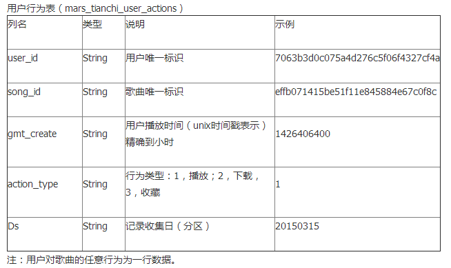
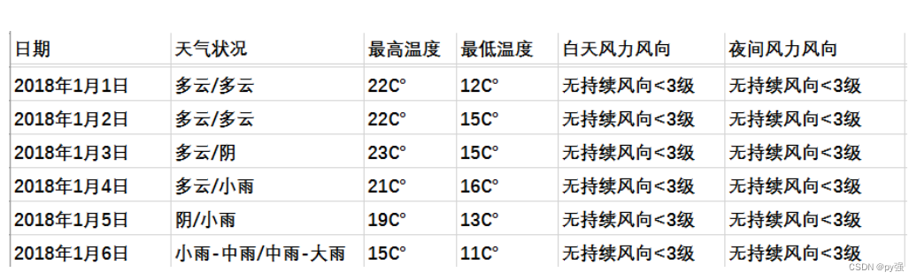
官方给的“输入”:2张表,一张是用户行为表(时间跨度20150301-20150830)mars_tianchi_user_actions,主要描述用户对歌曲的收藏,下载,播放等行为,一张是歌曲信息表mars_tianchi_songs,主要用来描述歌曲所属的艺人,及歌曲的相关信息,如发行时间,初始热度,语言等。
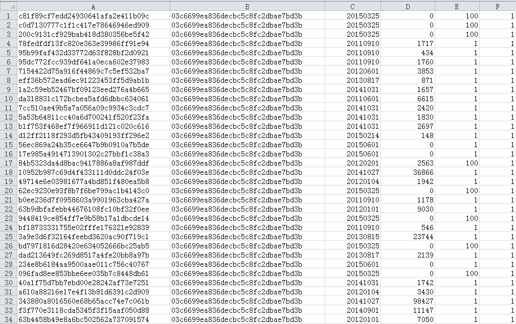
样例:
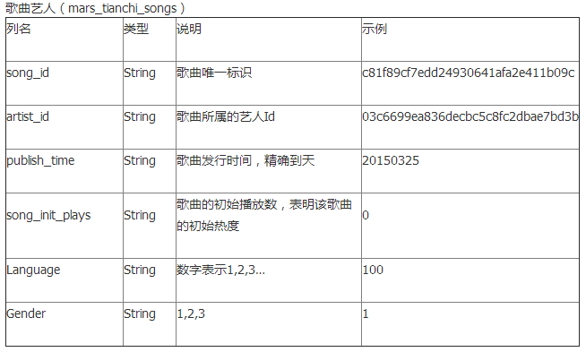
样例:
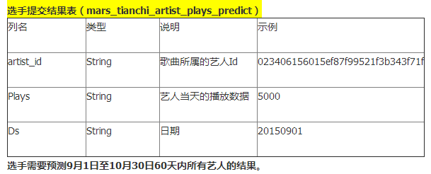
官方要求“输出”:预测随后2个月(20150901-20151030)每个歌手每天的播放量。输出格式:
2.初赛所用模型思路
由于是对歌手的播放量进行预测,所以直接对每个歌手的“播放量”这一对象进行统计,查看在20150301-20151030这8个月内歌手的播放量变化趋势,并以每天的播放量,连续3天的播放均值,连续3天的播放方差,作为一个时间点的样本,“滑动”构建神经网络的训练集。网络的构成如下:
(1)输入层:3个神经元,分别代表播放量,播放均值,播放方差;
(2)第一隐层:LSTM结构单元,带有35个LSTM单元;
(3)第二隐层:LSTM结构单元,带有10个LSTM单元;
(4)输出层:3个神经元,代表和输入层相同的含义。
目标函数:重构误差。
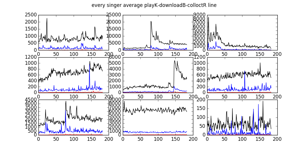
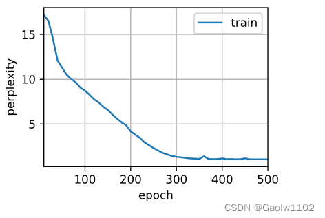
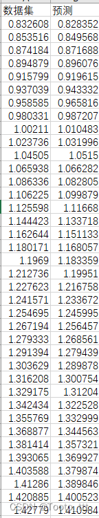
下图是某些歌手的播放统计曲线:
2.预测结果
蓝色代表歌手真实的播放曲线,绿色代表预测曲线:
三、代码
运行环境:windows下的spyder
语言:python 2.7,以及Keras深度学习库。
由于看这个赛题前,没有一点Python基础,所以也是边想思路边学Python,对Python中的数据结构不怎么了解,所以代码写得有点烂。但整个代码是可以运行无误的。这也是初赛时代码的最终版本。
# -*- coding: utf-8 -*-
"""
Created on Wed Jun 01 16:34:45 2016@author: Richer
"""
#%%修改记录
#1.将最后一层激活函数改为线性
#2.歌手播放曲线以歌曲量均值化(被第 4 点替换掉了)
#3.加入均值滤波 和 均值特征
#4.分别对每个歌手进行归一化处理(每个歌手之间相差太大了)
#5.对歌手进行聚类(效果不好)#%% 时间序列及字典
from __future__ import division
import pandas as pd
import pdb
#import time_DEBUG = False
_ISTEST = FalsetempList = pd.date_range(start = '20150301',end = '20150830')
i = 0
dateList = [] #给出的数据集所在的时间序列
while i < len(tempList):strTemp = str(tempList[i])[:10]strTemp = strTemp.replace('-','')dateList.append(strTemp)i = i + 1
recDict = {}.fromkeys(dateList,0) # 给出的数据集所在的时间序列字典
del tempList,i,strTemp tempList = pd.date_range(start = '20150831', end = '20151030')
i = 0
objDateL = [] #要预测的目标时间序列
while i < len(tempList):strTemp = str(tempList[i])[:10]strTemp = strTemp.replace('-','')objDateL.append(strTemp)i += 1
del strTemp, i## 异常数据信息
newSongExcep = 0 # 用户表中出现的新歌曲
userDsExcep = 0 # 用户表行为不在20150301-20150830#%% 表处理---歌曲艺人数据from copy import deepcopy
fileSong = open("p2_mars_tianchi_songs.csv")
songData = fileSong.readlines()bigSongDict = {} # 以歌曲为中心的大表
for songInfo in songData:songInfo = songInfo.replace('\n','')arrayInfo = songInfo.split(',')bigSongDict[arrayInfo[0]] = {} # 注:此处需要初始化,否则会出错bigSongDict[arrayInfo[0]]['artist_id'] = arrayInfo[1]bigSongDict[arrayInfo[0]]['publish_time'] = arrayInfo[2]bigSongDict[arrayInfo[0]]['song_init_plays'] = arrayInfo[3]bigSongDict[arrayInfo[0]]['Language'] = arrayInfo[4]bigSongDict[arrayInfo[0]]['Gender'] = arrayInfo[5]bigSongDict[arrayInfo[0]]['nUser'] = 0 #用户数目bigSongDict[arrayInfo[0]]['playRec'] = deepcopy(recDict) #播放记录bigSongDict[arrayInfo[0]]['downloadRec'] = deepcopy(recDict) #下载记录bigSongDict[arrayInfo[0]]['colloctRec'] = deepcopy(recDict) #收藏记录fileSong.close()
del songData,arrayInfo,songInfo# 用户行为数据fileUser = open("p2_mars_tianchi_user_actions.csv")
userData = fileUser.readlines()for userInfo in userData:userInfo = userInfo.replace('\n','')arrUser = userInfo.split(',')if (arrUser[1] in bigSongDict):bigSongDict[arrUser[1]]['nUser'] += 1if arrUser[3] == '1':bigSongDict[arrUser[1]]['playRec'][arrUser[4]] += 1if arrUser[3] == '2':bigSongDict[arrUser[1]]['downloadRec'][arrUser[4]] += 1if arrUser[3] == '3':bigSongDict[arrUser[1]]['colloctRec'][arrUser[4]] += 1else:newSongExcep = newSongExcep + 1fileUser.close()
del userData,userInfo,arrUser#%%统计每个艺人的播放,下载,收藏的变化曲线(20150301-20150830)from collections import Counter
singerDict = {} #歌手信息统计
for songKey in bigSongDict.keys():theArtist = bigSongDict[songKey]['artist_id']if (theArtist in singerDict):
# dict(Counter())会把 0 值去掉 # 对应的 key 相加singerDict[theArtist]['playRec'] = dict(Counter(singerDict[theArtist]['playRec']) + Counter(bigSongDict[songKey]['playRec'])) singerDict[theArtist]['downloadRec'] = dict(Counter(singerDict[theArtist]['downloadRec']) + Counter(bigSongDict[songKey]['downloadRec']))singerDict[theArtist]['colloctRec'] = dict(Counter(singerDict[theArtist]['colloctRec']) + Counter(bigSongDict[songKey]['colloctRec']))singerDict[theArtist]['nSongs'] += 1else:singerDict[theArtist] = {}singerDict[theArtist]['playRec'] = deepcopy(bigSongDict[songKey]['playRec'])singerDict[theArtist]['downloadRec'] = deepcopy(bigSongDict[songKey]['downloadRec'])singerDict[theArtist]['colloctRec'] = deepcopy(bigSongDict[songKey]['colloctRec'])singerDict[theArtist]['nSongs'] = 1#%%将singerDict中字典转换为序列-按日期排序import numpy as np
singerInfoList = {}
tpPlayList = [] # 播放列表
tpDownList = [] # 下载列表
tpCollectList = [] # 收藏列表
artList = [] # 歌手列表i = 0for singer in singerDict.keys():artList.append(singer)singerInfoList[singer] = {}#numSongs = singerDict[singer]['nSongs'] #对应歌手的歌曲数量while i < len(dateList):if (dateList[i] in singerDict[singer]['playRec'].keys()):tpPlayList.append(singerDict[singer]['playRec'][dateList[i]])else:tpPlayList.append(0)if (dateList[i] in singerDict[singer]['downloadRec'].keys()):tpDownList.append(singerDict[singer]['downloadRec'][dateList[i]])else:tpDownList.append(0)if(dateList[i] in singerDict[singer]['colloctRec'].keys()):tpCollectList.append(singerDict[singer]['colloctRec'][dateList[i]])else:tpCollectList.append(0)i += 1i = 0meanPlays = np.mean(tpPlayList)stdPlays = np.std(tpPlayList)singerInfoList[singer]['meanPlay'] = meanPlayssingerInfoList[singer]['stdPlay'] = stdPlayssingerInfoList[singer]['maxPlay'] = (abs((np.array(tpPlayList) - meanPlays) / stdPlays)).max()singerInfoList[singer]['playRec'] = deepcopy(tpPlayList)singerInfoList[singer]['downloadRec'] = deepcopy(tpDownList)singerInfoList[singer]['colloctRec'] = deepcopy(tpCollectList)del tpPlayList, tpDownList, tpCollectListtpPlayList = []tpDownList = []tpCollectList = []del tpPlayList, tpDownList, tpCollectList, singer,meanPlays,stdPlays#%%对每个歌手的播放曲线进行FFT变换
import matplotlib.pyplot as plt
import math#i = 0
#if _ISTEST == True:
# while i < len(singerInfoList):
# flagY = i % 9
# if flagY ==0:
# plt.figure(figsize = (10,8), dpi = 150)
# plt.suptitle('FFT process')
# plt.subplot(3,3,flagY + 1)
# fAmp = np.fft.fft(singerInfoList[artList[i]]['playRec']) / len(dateList)
# plt.stem(abs(fAmp[1:(len(fAmp)/2)]))
# i += 1
# del fAmp
#
#pdb.set_trace()#predictTestFFT = {} #使用FFT回归预测结果
#playLth = 0 #选取播放序列的长度做FFT
#chsNum = np.ones(len(singerInfoList),dtype=np.int) * 1 #选择前10个峰值做趋势预测
##chsNum[0] = 10
##chsNum[5] = 10
##chsNum[7] = 10
##chsNum[8] = 10
##chsNum[10] = 10
##chsNum[17] = 10
##chsNum[21] = 10
##chsNum[22] = 10
#
#if _ISTEST == True:
# playLth = len(dateList) - len(objDateL)
#else:
# playLth = len(dateList)
#
#j = 0 #歌手索引
#i = 0 #FFT索引
#while j < len(singerInfoList):
# i = 0
# ampFFT = np.fft.fft(singerInfoList[artList[j]]['playRec'][:playLth]) / playLth
# sortInd = sorted(xrange(len(ampFFT)),key = (abs(ampFFT)).__getitem__,reverse = True) #降序排列
# chsAmp = np.zeros(chsNum[j])
# while i < chsNum[j]:
# chsAmp[i] = ampFFT[sortInd[i]]
# i += 1
# dateRcon = np.zeros((playLth + len(objDateL)))
# ind = np.arange(0,len(dateRcon),1.0) / len(ampFFT) * (2 * np.pi)
# for k, p in enumerate(chsAmp):
# if k != 0:
# p *= 2
# dateRcon += np.real(p) * np.cos(k * ind)
# dateRcon -= np.imag(p) * np.sin(k * ind)
# predictTestFFT[artList[j]] = {}
# predictTestFFT[artList[j]]['playRec'] = deepcopy((list(dateRcon))[playLth:(playLth + len(objDateL))])
#
# if _ISTEST == True:
# flagY = j % 9
# if flagY == 0:
# plt.figure(figsize = (10,8),dpi = 150)
# plt.suptitle('predict test play - use fft')
# plt.subplot(3,3,flagY + 1)
# plt.plot(singerInfoList[artList[j]]['playRec'][playLth:(playLth + len(objDateL))],'b')
# plt.plot(predictTestFFT[artList[j]]['playRec'],'g')
# j += 1
# del ampFFT,sortInd,chsAmp,dateRcon,ind
#
#
#pdb.set_trace()#%% 绘制歌手播放,下载,收藏曲线xVal = range(len(dateList)) #x坐标值
i = 0while i < len(singerInfoList): # 每个歌手播放曲线flagY = i % 9if flagY == 0:plt.figure(figsize = (10,8), dpi = 150)plt.suptitle('every singer average playK-downloadB-colloctR line')plt.subplot(3,3,flagY + 1)plt.plot(singerInfoList[artList[i]]['playRec'],'k')plt.plot(singerInfoList[artList[i]]['downloadRec'],'b')plt.plot(singerInfoList[artList[i]]['colloctRec'],'r')i += 1del flagY#%%提取歌手的标准差信息并进行排序#nCls = 1 #分类数
#clsTh = 0 #第几类
#
#nSgrToCls = [] #每类的歌手数量列表
#stdPlayList = [] #所有歌手标准差列表
#indStdList = [] #排序后的数据在原始序列中的索引
#
#i = 0
#while i < len(artList):
# stdPlayList.append(singerInfoList[artList[i]]['stdPlay'])
# i += 1
#
#indStdList = sorted(xrange(len(stdPlayList)),key = stdPlayList.__getitem__) #默认降序排列
#
#i = 0
#while i < (nCls - 1):
# nSgrToCls.append(int(len(singerInfoList) / nCls))
# i += 1
#if nCls == 1:
# nSgrToCls.append(int(len(singerInfoList)))
#else:
# nSgrToCls.append(int(len(singerInfoList) - (nCls - 1) * nSgrToCls[0]))
#
#nObjSgr = nSgrToCls[clsTh] #目标歌手数量
#objInd = [] #初始化-对应的索引
#if clsTh == (nCls -1):
# objInd = indStdList[( (nCls - 1) * nSgrToCls[0] ):]
#else:
# objInd = indStdList[(clsTh * nSgrToCls[0]):((clsTh + 1) * nSgrToCls[0])]nObjSgr = len(singerInfoList)
objInd = range(nObjSgr)#%% 将singerDict 的 playRec downloadRec colloctRec按时间顺序转换为list
# 且分别对每个歌手数据进行归一化playList = [] #大播放列表
downList = [] # 大下载列表
collectList = [] #大收藏列表
avePlayList = [] # 播放曲线的均值滤波后曲线
varPlayList = [] #实际上是标准差曲线i = 0
while i < nObjSgr:artSg = artList[objInd[i]] meanPlays = singerInfoList[artSg]['meanPlay']stdPlays = singerInfoList[artSg]['stdPlay']maxPlays = singerInfoList[artSg]['maxPlay']playList = playList + list( (np.array(singerInfoList[artSg]['playRec']) - meanPlays) / (stdPlays * maxPlays) )downList = downList + singerInfoList[artSg]['downloadRec']collectList = collectList + singerInfoList[artSg]['colloctRec']i += 1
del meanPlays,stdPlays,maxPlays,artSg#所有歌手的播放下载收藏曲线放在一起
plt.figure(figsize = (10,8), dpi = 150)
plt.plot(playList,'k')
plt.plot(downList,'b')
plt.plot(collectList,'r')
plt.title('overall playK-downB-colloctR')#相关参数(影响结果的重要参数)
seqLength = 10 #序列长度
testSetRate = 0 #测试集比例
if _ISTEST == True:testSetRate = len(objDateL) / len(dateList)
else:testSetRate = 0
lenDate = len(dateList) #给定的数据集时间长度
nSinger = nObjSgr #len(singerInfoList) #艺人数量
batchSize = 50
validRate = 0.2
aveFilter = 4 # 均值滤波长度in_out_neurons = 3 #输入输出神经元个数
firLSTM = 35 #第一层神经元个数
secLSTM = 10 #第二层神经元个数
epochD = 600 #迭代次数#%%对播放曲线列表 playList 进行均值滤波 及 求取标准差曲线i = 0
while i < nSinger:j = i * lenDatefj = i * lenDate #起点ej = (i + 1) * lenDate #终点while j < ej:if j < (i * lenDate + aveFilter -1):avePlayList.append(np.mean(playList[fj:(j+1)]))varPlayList.append(np.std(playList[fj:(j+1)]))else:avePlayList.append(np.mean(playList[(j-aveFilter+1):(j+1)]))varPlayList.append(np.std(playList[(j-aveFilter+1):(j+1)]))j +=1i +=1#均值滤波结果显示
i = 0
while i < nSinger:flagY = i % 9if flagY == 0:plt.figure(figsize = (10,8), dpi =150)plt.suptitle('average filter-play-originalK filterB')plt.subplot(3,3,flagY + 1)stPt = i * lenDateendPt = (i + 1) * lenDateplt.plot(playList[stPt:endPt],'k')plt.plot(avePlayList[stPt:endPt],'b')i += 1dateSet = pd.DataFrame({"avePlay":avePlayList,"play":playList,"varPlay":varPlayList}) #全体数据集
dateSet.to_csv("originalDataSet.csv")
dateSetOrigin = deepcopy(dateSet) # 原始数据集保存一份# 数据预处理 去均值 方差归一 缩放到[-1 1]
#if _DEBUG == True:
# pdb.set_trace()#avePlayMean = dateSet['avePlay'].mean()
##downMean = dateSet['down'].mean()
#playMean = dateSet['play'].mean()
#
#dateSet['avePlay'] = dateSet['avePlay'] - avePlayMean
##dateSet['down'] = dateSet['down'] - downMean
#dateSet['play'] = dateSet['play'] - playMean
#
#avePlayStd = dateSet['avePlay'].std()
##downStd = dateSet['down'].std()
#playStd = dateSet['play'].std()
#
#dateSet['avePlay'] = dateSet['avePlay'] / avePlayStd
##dateSet['down'] = dateSet['down'] / downStd
#dateSet['play'] = dateSet['play'] / playStd
#
#factorMax = abs(dateSet).max().max() + 0.05
#
#dateSet = dateSet / factorMax
#dateSet.to_csv("preproceeDataSet.csv")#所有歌手的播放曲线
plt.figure(figsize = (10,8), dpi = 150)
plt.plot(dateSet['play'],'k')
plt.plot(dateSet['avePlay'],'b')
plt.plot(dateSet['varPlay'],'g')
plt.xlabel('index')
plt.ylabel('playK-avePlayB')
plt.title('overall playK-avePlayB-varPlayG - preprocessed')#%%训练集测试集划分
def load_data(data, n_prev = 14): docX, docY = [], []for i in range(len(data)-n_prev):
# pdb.set_trace()docX.append(data.iloc[i:i+n_prev].as_matrix())docY.append(data.iloc[i+n_prev].as_matrix())
# alsX = np.array(docX)
# alsY = np.array(docY)return docX, docYdef train_test_split(df, test_size = 1 / 3, seqL = 14): ntrn = int(round(len(df) * (1 - test_size)))X_train, y_train = load_data(df.iloc[0:ntrn],seqL)X_test, y_test = load_data(df.iloc[ntrn:],seqL)return (X_train, y_train), (X_test, y_test)# 训练集 测试集 划分
if _DEBUG == True:pdb.set_trace()
#初值
(xTrain,yTrain), (xTest,yTest) = train_test_split(dateSet[0:lenDate],testSetRate,seqLength)needPredict = [] # 需要被预测的后续序列的真实值
tempIndex = int(round(lenDate * (1 - testSetRate)))
if _ISTEST == True:needPredict.append(dateSet[0:lenDate].iloc[tempIndex:].as_matrix()) # 三维数组,每组是一个歌手需要预测的序列i = 1while i < nSinger:startPt = i * lenDateendPt = (i + 1) * lenDatetempData = dateSet[startPt:endPt](xTrainTp,yTrainTp), (xTestTp,yTestTp) = train_test_split(tempData,testSetRate,seqLength)xTrain = np.vstack((xTrain,xTrainTp))yTrain = np.vstack((yTrain,yTrainTp))xTest = np.vstack((xTest,xTestTp))yTest = np.vstack((yTest,yTestTp))tempIndex = int(round(len(tempData) * (1 - testSetRate)))if _ISTEST == True:needPredict.append(tempData.iloc[tempIndex:].as_matrix())i += 1X_Train = np.array(xTrain)
Y_Train = np.array(yTrain)
X_Test = np.array(xTest)
Y_Test = np.array(yTest)del xTrain, yTrain, xTest, yTest#%%绘制需要被预测的数据之间的差异
if _ISTEST == True:i = 0plt.figure(figsize = (10,8), dpi = 150)while i < nSinger:orgValue = pd.DataFrame(needPredict[i])plt.plot(orgValue[1])i += 1del orgValueplt.suptitle('need predict test data - preprocess data')#%% 训练算法模型
if _DEBUG == True:pdb.set_trace()from keras.models import Sequential
from keras.layers.core import Dense, Activation
from keras.layers.recurrent import LSTM
from keras.callbacks import EarlyStoppingmodel = Sequential()
# LSTM作为第一层---输入层维度:input_dim,输出层维度:hidden_neurons
model.add(LSTM(firLSTM, input_dim=in_out_neurons, input_length=seqLength,return_sequences=True))
model.add(LSTM(secLSTM,return_sequences=False))
#model.add(LSTM(thiLSTM))
# 标准的一维全连接层---输出:in_out_neurons,输入:input_dim
model.add(Dense(in_out_neurons,activation='linear'))
model.compile(loss="mse", optimizer="rmsprop") # mse mean_squared_error
#提前中断训练
earlyStopping = EarlyStopping(monitor = 'val_loss', patience = 10)
# X_Train三维数组,每组是一个序列
hist = model.fit(X_Train, Y_Train, batch_size=batchSize, nb_epoch=epochD, verbose=0, shuffle = False,validation_split=validRate,callbacks = [earlyStopping])
#print(hist.history)#对训练集进行预测-调试用
predictTrain = model.predict(X_Train) # 二维数组,每一行是一组预测值
predictDF = pd.DataFrame(predictTrain)
Y_TrainDF = pd.DataFrame(Y_Train)plt.figure(figsize = (10,8), dpi = 150)
plt.plot(list(predictDF[1]),'g')
plt.plot(list(Y_TrainDF[1]),'b')
plt.title('train set predict check')if _DEBUG == True:pdb.set_trace()#%%预测
i = 0
j = 0
predictTest = {} # 所有歌手最终预测结果
while j < nSinger:artSg = artList[objInd[j]]predictTest[artSg] = {}predictTest[artSg]['playRec'] = [] predictTest[artSg]['avePlay'] = [] predictTest[artSg]['varPlay'] = []j += 1
del artSgif _DEBUG == True:pdb.set_trace()
i = 0
j = 0
lastIndex = len(X_Train) / nSinger
while j < nSinger:lastData = np.array([X_Train[int(lastIndex * (j+1) -1)]])while i < len(objDateL): #预测天数predictTp = model.predict(lastData)artSg = artList[objInd[j]]predictTest[artSg]['varPlay'].append(predictTp[0][2])predictTest[artSg]['playRec'].append(predictTp[0][1])predictTest[artSg]['avePlay'].append(predictTp[0][0])lastData = np.array([np.vstack((lastData[0][1:],predictTp))])i += 1j += 1i = 0del lastData, predictTp
del artSg# 预测结果分析---数据还原之前
i = 0
xIndex = range(len(objDateL))
if _ISTEST == True:while i < nSinger: # 播放预测曲线flagY = i % 9if flagY == 0:plt.figure(figsize = (10,8), dpi = 150)plt.suptitle('test set: predict play')plt.subplot(3,3,flagY + 1)orgValue = pd.DataFrame(needPredict[i]) # needPredict三维数组,每组是一个歌手需要预测的序列值artSg = artList[objInd[i]]plt.plot(xIndex,predictTest[artSg]['playRec'],'g')plt.plot(xIndex,orgValue[1],'b')i += 1del orgValuedel artSgi = 0
if _ISTEST == True:while i < nSinger: # 平均值预测曲线flagY = i % 9if flagY == 0:plt.figure(figsize = (10,8), dpi = 150)plt.suptitle('test-predict avePlay')plt.subplot(3,3,flagY + 1)orgValue = pd.DataFrame(needPredict[i])artSg = artList[objInd[i]]plt.plot(xIndex,predictTest[artSg]['avePlay'],'g')plt.plot(xIndex,orgValue[0],'b')i += 1del orgValuedel artSg#i = 0
#while i <nSinger: # 收藏预测曲线
# flagY = i % 9
# if flagY == 0:
# plt.figure(figsize = (10,8), dpi = 150)
#
# plt.subplot(3,3,flagY +1)
# orgValue = pd.DataFrame(needPredict[i])
# plt.plot(xIndex,predictTest[artList[i]]['colloctRec'],'g')
# plt.plot(xIndex,orgValue[0],'b')
#
# i += 1
# del orgValue
#plt.suptitle('test-predict colloct')#%%预测---还原到原始数据集
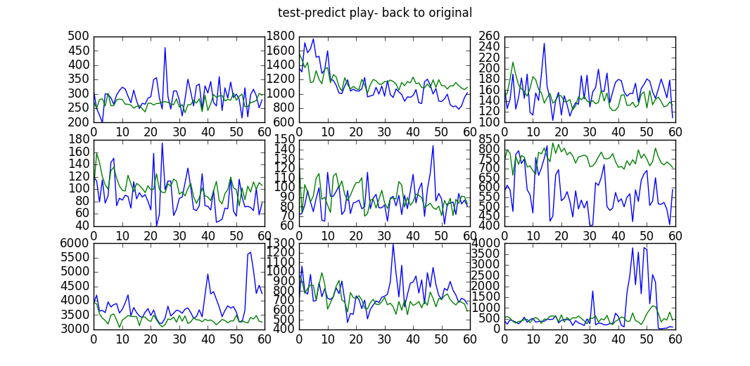
if _ISTEST == True:i = 0while i < nSinger:flagY = i % 9if flagY == 0:plt.figure(figsize = (10,8), dpi =150)plt.suptitle('test-predict play- back to original')plt.subplot(3,3,flagY + 1)artSg = artList[objInd[i]]meanPlays = singerInfoList[artSg]['meanPlay']stdPlays = singerInfoList[artSg]['stdPlay']maxPlays = singerInfoList[artSg]['maxPlay']orgValue = ((pd.DataFrame(needPredict[i]))[1]) * maxPlays * stdPlays + meanPlaysaftValue = ((pd.DataFrame(predictTest[artSg]['playRec']))[0]) * maxPlays * stdPlays + meanPlaysplt.plot(xIndex,orgValue,'b')plt.plot(xIndex,aftValue,'g')i +=1del orgValue, aftValuedel artSg#使用 aveplay 预测真实 play
if _ISTEST == True:i = 0while i < nSinger:flagY = i % 9if flagY == 0:plt.figure(figsize = (10,8), dpi =150)plt.suptitle('use avePlay to predict real play line')plt.subplot(3,3,flagY + 1)artSg = artList[objInd[i]]meanPlays = singerInfoList[artSg]['meanPlay']stdPlays = singerInfoList[artSg]['stdPlay']maxPlays = singerInfoList[artSg]['maxPlay']orgValue = ((pd.DataFrame(needPredict[i]))[1]) * maxPlays * stdPlays + meanPlaysaftValue = ((pd.DataFrame(predictTest[artSg]['avePlay']))[0]) * maxPlays * stdPlays + meanPlaysplt.plot(xIndex,orgValue,'b')plt.plot(xIndex,aftValue,'g')i +=1del orgValue, aftValuedel artSg#%%融合svr
svrResult = {}
fileSVR = open("svr.csv")
svrData = fileSVR.readlines()for svrInfo in svrData:svrInfo = svrInfo.replace('\n','')arrInfo = svrInfo.split(',')svrResult[arrInfo[0]] = int(arrInfo[1])fileSVR.close()
del svrData,svrInfo,arrInfo#%% 评价指标if _ISTEST == True:singerF = [] # 每个歌手的评价指标值 FsumF = 0i = 0while i < nSinger:artSg = artList[objInd[i]]meanPlays = singerInfoList[artSg]['meanPlay']stdPlays = singerInfoList[artSg]['stdPlay']maxPlays = singerInfoList[artSg]['maxPlay']orgValue = ((pd.DataFrame(needPredict[i]))[1]) * maxPlays * stdPlays + meanPlaysaftValue = ((pd.DataFrame(predictTest[artSg]['playRec']))[0]) * maxPlays * stdPlays + meanPlaystempArr = (np.array(aftValue) - np.array(orgValue)) / (np.array(orgValue))tempS = ((tempArr * tempArr).sum()) / len(objDateL)theta = math.sqrt(tempS)tempFi = math.sqrt((np.array(orgValue)).sum())sumF = sumF + (1-theta) * tempFisingerF.append((1-theta) * tempFi)i += 1del orgValue,aftValue,tempArrdel artSgif _ISTEST == True:singerFA = [] # 每个歌手的评价指标值 FsumF = 0i = 0while i < nSinger:artSg = artList[objInd[i]]meanPlays = singerInfoList[artSg]['meanPlay']stdPlays = singerInfoList[artSg]['stdPlay']maxPlays = singerInfoList[artSg]['maxPlay']orgValue = ((pd.DataFrame(needPredict[i]))[1]) * maxPlays * stdPlays + meanPlaysaftValue = (((pd.DataFrame(predictTest[artSg]['playRec']))[0]) * maxPlays * stdPlays + meanPlays) * 0.5 + svrResult[artSg] * 0.5tempArr = (np.array(aftValue) - np.array(orgValue)) / (np.array(orgValue))tempS = ((tempArr * tempArr).sum()) / len(objDateL)theta = math.sqrt(tempS)tempFi = math.sqrt((np.array(orgValue)).sum())sumF = sumF + (1-theta) * tempFisingerFA.append((1-theta) * tempFi)i += 1del orgValue,aftValue,tempArrdel artSg
# resF = pd.DataFrame({"singerf":singerF})
# resF.to_csv("singerF.csv")#%%使用均值预测后的评价指标值
#singerF_AVG = [] # 每个歌手的评价指标值 F
#sumF = 0
#i = 0
#while i < nSinger:
# meanPlays = singerInfoList[artList[i]]['meanPlay']
# stdPlays = singerInfoList[artList[i]]['stdPlay']
# maxPlays = singerInfoList[artList[i]]['maxPlay']
#
# orgValue = ((pd.DataFrame(needPredict[i]))[1]) * maxPlays * stdPlays + meanPlays
# aftValue = ((pd.DataFrame(predictTest[artList[i]]['avePlay']))[0]) * maxPlays * stdPlays + meanPlays
#
# tempArr = (np.array(aftValue) - np.array(orgValue)) / (np.array(orgValue))
# tempS = ((tempArr * tempArr).sum()) / len(objDateL)
# theta = math.sqrt(tempS)
#
# tempFi = math.sqrt((np.array(orgValue)).sum())
# sumF = sumF + (1-theta) * tempFi
#
# singerF_AVG.append((1-theta) * tempFi)
#
# i += 1
# del orgValue,aftValue,tempArr
#sum(singerF_AVG[:36]) + sum(singerF_AVG[37:56]) + sum(singerF_AVG[57:])#%%写入到预测文件
if _ISTEST == False:import csvresFile = open("mars_tianchi_artist_plays_predict.csv","wb")writerRes = csv.writer(resFile)i = 0j = 1while i < nSinger:artSg = artList[objInd[i]]meanPlays = singerInfoList[artSg]['meanPlay']stdPlays = singerInfoList[artSg]['stdPlay']maxPlays = singerInfoList[artSg]['maxPlay']aftValue = (((pd.DataFrame(predictTest[artSg]['playRec']))[0]) * maxPlays * stdPlays + meanPlays) * 0.5 + svrResult[artSg] * 0.5while j < len(objDateL):oneLineData = [artSg,str(int(aftValue[j])),objDateL[j]]writerRes.writerow(oneLineData)del oneLineDataj += 1del aftValuej = 1i += 1resFile.close()del artSg
四、参考文献
1.LSTM入门介绍比较好的文章:A Critical review of rnn for sequence learning
2.LSTM学习思路,参见知乎的一个介绍,很详细:https://www.zhihu.com/question/29411132 。
3.Python入门视频教程—可看南京大学张莉老师在coursera上的公开课《用Python玩转数据》,有例子介绍,很实用。https://www.coursera.org/learn/hipython/home/welcome。
4.Keras介绍—参看官方文档http://keras.io/

![人人都能用Python写出LSTM-RNN的代码![你的神经网络学习最佳起步]](https://img-blog.csdnimg.cn/img_convert/cfca0b70e6d14e6cd1e0ae5c87f3b8aa.png)


![[深入浅出] LSTM神经网络](https://img-blog.csdnimg.cn/img_convert/d9fa736dddf779de72df0c72172cf225.png)