python中的分位数回归（初探）

分位数回归

参考文献

Python statsmodels 介绍 - 树懒学堂 (shulanxt.com)

Quantile Regression - IBM Documentation

https://www.cnblogs.com/TMesh/p/11737368.html

传统的线性回归模型

其的求解方式是一个最小二乘法，保证观测值与你的被估值的差的平方和应该保持最小，
$MSE\ =\ \frac{1}{n}\sum_{i=1}^n{\left( y_i-\widehat{f}\left( x_i \right) \right) ^2\ =\ E\left( y-\widehat{f}\left( x \right) \right)}^2$

因变量的条件均值分布受自变量x的影响过程，因此我们拟合出来的曲线是在给定x的情况下，y的条件均值
随机误差项来均值为0、同方差，因此估计的斜率在现有的基础上是最好的

分位数回归

首先提出中位数回归（最小绝对偏差估计）
改进出分位数回归
描述自变量X对因变量Y的变化范围，以及其不受分布形状的影响。即其不止可以描述条件均值的影响，还可以描述中位数的影响

因此我们能够得到如下的一个损失函数
$\widehat{Q_Y}\left( \tau \right) =arg\min _{\xi _{r\in R}}\left( \sum_{i:Y_i\ge \xi _{t^{au}}}{\tau \left| Y_i-\xi _r \right|}+\sum_{i:Y_i<\xi _{t^{au}}}{\left( 1-\tau \right) \left| Y_i-\xi _r \right|} \right)$
参数 $\tau$ 的估计算法有：

单纯形算法
内点算法
平滑算法

总结来说，在我心目中，分位数回归是对传统回归的一种改进，它不在局限于原来最小二乘法，使得数据可以更多影响其他的点或者类似于中位数的影响。

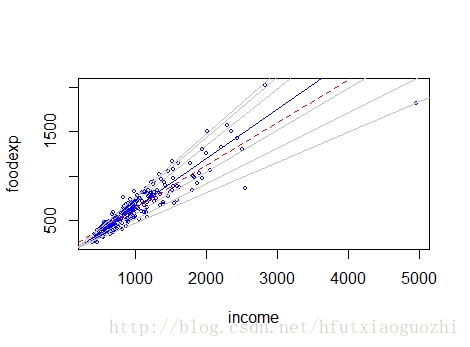
接下来我们将采用python语言进行实现，采用的数据集是我们之前的文章中cpu—time_tamp的数据

class QuantileRegression:def __init__(self,data):# self.data = pd.DataFrame(data=np.hstack([time_stamp,cpu_util_percent]),columns=["time_stamp","cpu_util_percent"])self.data = data# self.num = len(time_stamp)passdef __QuantileReq_1__(self):# 主义这里，前面是Y轴，后面是X轴mod = smf.quantreg('cpu_util_percent~time_stamp',self.data)print(mod)res = mod.fit()print(res)fig = plt.subplots(figsize=(8, 6))# x = np.arange(self.data.time_stamp.min(),self.data.time_stamp.max(),1000)print(res.summary())

在这里插入图片描述

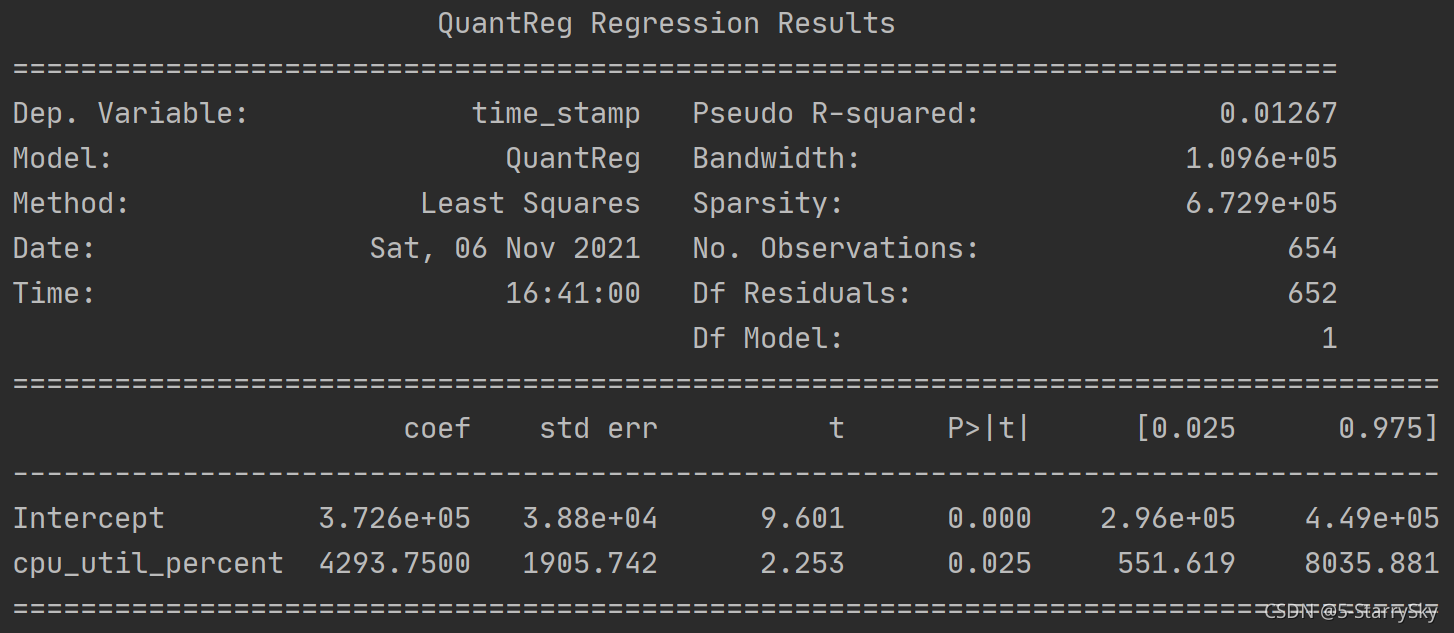
数据解释：

Dep. Variable ：因变量
Model：方法模块
Method：方法（最小二乘法）默认使用迭代加权最小二乘法（IRLS）
Date:日期
Time：时间
Pseudo R-squared: 拟合优度

采用的公式为：
$R_{q}^{2}=1-\frac{\sum_{i=1}^{n} \rho_{q}\left(y_{i}-x_{i}^{\prime} \beta\right)}{\sum_{i=1}^{n} \rho_{q}\left(y_{i}-y_{q}\right)}$
Bandwidth：窗宽h

公式来源于：
$y_{i}>x_{i}^{\prime} \beta , d_{i}=\left[\frac{q}{f(0)}\right]^{2} , 当 y_{i} \leq x_{i}^{\prime} \beta ， d_{i}=\left[\frac{1-q}{f(0)}\right]^{2} f(0)_{\text {的估计为 }} \tilde{f(0)}=\frac{1}{n} \sum_{i=1}^{n} \frac{1}{h} K\left[\frac{e_{i}}{h}\right]$

$f(0)_{\text {的估计为 }} \tilde{f(0)}=\frac{1}{n} \sum_{i=1}^{n} \frac{1}{h} K\left[\frac{e_{i}}{h}\right] 其中e_i=y_i-x_{i}^{'}\beta ,K[]表示为核函数$
Sparsity
No. Observations：
Df Residuals ：Df残差
Df Model
coef：系数
std err：协方差（标准差）

采用以下公式得到：
$Asy.\operatorname{Var}\left[\beta_{q}\right]=\left(X^{\prime} X\right)^{-1} X^{\prime} D X\left(X^{\prime} X\right)^{-1} $ 其中D为对角矩阵，
t：统计量，表示为 $\dfrac{\widetilde{\beta }}{Va\tilde{r}}\left( \beta \right)$
P>|t|
[0.025 0.975]
Intercept：截距
cpu_util_percent ：斜率

但在多次实验的过程中，发现一直报过时未收敛的警告，所以我查看了源代码，最终我们怀疑python的分位数回归可能不太适用于曲线回归，可能只能分段式线性回归比较合适，以下是源代码的部分

#!/usr/bin/env python'''
Quantile regression modelModel parameters are estimated using iterated reweighted least squares. The
asymptotic covariance matrix estimated using kernel density estimation.Author: Vincent Arel-Bundock
License: BSD-3
Created: 2013-03-19The original IRLS function was written for Matlab by Shapour Mohammadi,
University of Tehran, 2008 (shmohammadi@gmail.com), with some lines based on
code written by James P. Lesage in Applied Econometrics Using MATLAB(1999).PP.
73-4.  Translated to python with permission from original author by Christian
Prinoth (christian at prinoth dot name).
'''import numpy as np
import warnings
import scipy.stats as stats
from numpy.linalg import pinv
from scipy.stats import norm
from statsmodels.tools.decorators import cache_readonly
from statsmodels.regression.linear_model import (RegressionModel,RegressionResults,RegressionResultsWrapper)
from statsmodels.tools.sm_exceptions import (ConvergenceWarning,IterationLimitWarning)[docs]class QuantReg(RegressionModel):# 计算回归系数及其协方差矩阵。q是分位数，vcov是协方差矩阵，默认robust即2.5的方法，核函数kernel默认# epa,窗宽bandwidth默认hsheather.IRLS最大迭代次数默认1000，差值默认小于1e-6时停止迭代'''Quantile Regression使用迭代加权最小二乘法估计分位数回归模型。Estimate a quantile regression model using iterative reweighted leastsquares.Parameters----------endog : array or dataframe   数据/数据帧endogenous/response variable  内源性/响应变量exog : array or dataframeexogenous/explanatory variable(s) 外生/解释变量(s)Notes-----The Least Absolute Deviation (LAD) estimator is a special case wherequantile is set to 0.5 (q argument of the fit method).最小绝对偏差(LAD)估计量是一种特殊情况Quantile被设置为0.5 (fit方法的q参数)。The asymptotic covariance matrix is estimated following the procedure inGreene (2008, p.407-408), using either the logistic or gaussian kernels(kernel argument of the fit method).在此基础上，对渐近协方差矩阵进行了估计格林(2008,p.407-408)，使用logistic或高斯核(拟合方法的核心参数)。References----------General:* Birkes, D. and Y. Dodge(1993). Alternative Methods of Regression, John Wiley and Sons.* Green,W. H. (2008). Econometric Analysis. Sixth Edition. International Student Edition.* Koenker, R. (2005). Quantile Regression. New York: Cambridge University Press.* LeSage, J. P.(1999). Applied Econometrics Using MATLAB,* Birkes, D.和Y. Dodge(1993)。回归的可选方法，约翰·威利和儿子。* Green,W。h(2008)。计量经济学分析。第六版。国际学生版。* Koenker, R.(2005)。分位数回归。纽约:剑桥大学出版社。* LeSage J. P.(1999)。应用计量经济学Kernels (used by the fit method):* Green (2008) Table 14.2Bandwidth selection (used by the fit method):* Bofinger, E. (1975). Estimation of a density function using order statistics. Australian Journal of Statistics 17: 1-17.* Chamberlain, G. (1994). Quantile regression, censoring, and the structure of wages. In Advances in Econometrics, Vol. 1: Sixth World Congress, ed. C. A. Sims, 171-209. Cambridge: Cambridge University Press.* Hall, P., and S. Sheather. (1988). On the distribution of the Studentized quantile. Journal of the Royal Statistical Society, Series B 50: 381-391.Keywords: Least Absolute Deviation(LAD) Regression, Quantile Regression,Regression, Robust Estimation.* Bofinger E.(1975)。使用顺序统计量估计密度函数。澳大利亚统计杂志17:1-17。*张伯伦，G.(1994)。分位数回归、审查和工资结构。《计量经济学进展》，第1卷:第六届世界大会，c.a.西姆斯编，171-209。剑桥:剑桥大学出版社。* Hall, P.和S. Sheather。(1988)。研究分位数的分布。皇家统计学会学报，B辑50:381-391。关键词:最小绝对偏差回归分位数回归回归,稳健估计。'''# 初始化def __init__(self, endog, exog, **kwargs):self._check_kwargs(kwargs)super(QuantReg, self).__init__(endog, exog, **kwargs)[docs]    def whiten(self, data):"""QuantReg model whitener does nothing: returns data.QuantReg模型增白器什么也不做:返回数据。"""return data[docs]    def fit(self, q=.5, vcov='robust', kernel='epa', bandwidth='hsheather',max_iter=1000, p_tol=1e-6, **kwargs):"""Solve by Iterative Weighted Least Squares用迭代加权最小二乘法求解Parameters----------q : floatQuantile must be strictly between 0 and 1vcov : str, method used to calculate the variance-covariance matrixof the parameters. Default is ``robust``:- robust : heteroskedasticity robust standard errors (as suggestedin Greene 6th edition)- iid : iid errors (as in Stata 12)q:浮动型小数分位数必须严格在0和1之间vcoc:str，用于计算方差-协方差矩阵的参数方法。默认是“robust”:-robust:异方差鲁棒性标准误差(如在格林第六版中的建议)- iid: iid错误(如Stata 12)kernel : str, kernel to use in the kernel density estimation for theasymptotic covariance matrix:Kernel: str，用于核密度估计的渐近协方差矩阵的核:- epa: Epanechnikov- cos: Cosine  余旋- gau: Gaussian 高斯- par: Parzenebandwidth : str, Bandwidth selection method in kernel densityestimation for asymptotic covariance estimate (fullreferences in QuantReg docstring):bandwidth: str，渐近协方差估计核密度估计中的带宽选择方法(完整参考QuantReg文档字符串):- hsheather: Hall-Sheather (1988)- bofinger: Bofinger (1975)- chamberlain: Chamberlain (1994)"""if q <= 0 or q >= 1:raise Exception('q must be strictly between 0 and 1')kern_names = ['biw', 'cos', 'epa', 'gau', 'par']if kernel not in kern_names:raise Exception("kernel must be one of " + ', '.join(kern_names))else:kernel = kernels[kernel]if bandwidth == 'hsheather':bandwidth = hall_sheatherelif bandwidth == 'bofinger':bandwidth = bofingerelif bandwidth == 'chamberlain':bandwidth = chamberlainelse:raise Exception("bandwidth must be in 'hsheather', 'bofinger', 'chamberlain'")#endog样本因变量，exog样本自变量endog = self.endogexog = self.exognobs = self.nobsexog_rank = np.linalg.matrix_rank(self.exog)self.rank = exog_rankself.df_model = float(self.rank - self.k_constant)self.df_resid = self.nobs - self.rank#IRLS初始化n_iter = 0xstar = exogbeta = np.ones(exog.shape[1])# TODO: better start, initial beta is used only for convergence check# 待办事项:更好的开始，初始测试版仅用于收敛检查# Note the following does not work yet,# the iteration loop always starts with OLS as initial beta# if start_params is not None:#    if len(start_params) != rank:#       raise ValueError('start_params has wrong length')#       beta = start_params#    else:#       # start with OLS#       beta = np.dot(np.linalg.pinv(exog), endog)"""#注意以下内容还不能使用，迭代循环总是以OLS作为初始测试开始#如果start_params不是None:# if len(start_params) != rank:#引发ValueError('start_params has wrong length')# beta = start_params其他:# #从OLS开始# beta = np.dot(np. linalgr .pinv(exog)， endog)"""diff = 10cycle = Falsehistory = dict(params = [], mse=[])#IRLS迭代while n_iter < max_iter and diff > p_tol and not cycle:n_iter += 1beta0 = betaxtx = np.dot(xstar.T, exog)xty = np.dot(xstar.T, endog)beta = np.dot(pinv(xtx), xty)resid = endog - np.dot(exog, beta)mask = np.abs(resid) < .000001resid[mask] = ((resid[mask] >= 0) * 2 - 1) * .000001resid = np.where(resid < 0, q * resid, (1-q) * resid)resid = np.abs(resid)#1/resid[:, np.newaxis]为更新权重Wxstar = exog / resid[:, np.newaxis]diff = np.max(np.abs(beta - beta0))history['params'].append(beta)history['mse'].append(np.mean(resid*resid))#检查是否收敛，若收敛则提前停止迭代if (n_iter >= 300) and (n_iter % 100 == 0):# check for convergence circle, should not happenfor ii in range(2, 10):if np.all(beta == history['params'][-ii]):cycle = Truewarnings.warn("Convergence cycle detected", ConvergenceWarning)break# 超出迭代次数，发出警告并结束，迭代次数默认为1000if n_iter == max_iter:warnings.warn("Maximum number of iterations (" + str(max_iter) +") reached.", IterationLimitWarning)#计算协方差矩阵e = endog - np.dot(exog, beta)# Greene (2008, p.407) writes that Stata 6 uses this bandwidth:# h = 0.9 * np.std(e) / (nobs**0.2)# Instead, we calculate bandwidth as in Stata 12iqre = stats.scoreatpercentile(e, 75) - stats.scoreatpercentile(e, 25)h = bandwidth(nobs, q)h = min(np.std(endog),iqre / 1.34) * (norm.ppf(q + h) - norm.ppf(q - h))fhat0 = 1. / (nobs * h) * np.sum(kernel(e / h))if vcov == 'robust':d = np.where(e > 0, (q/fhat0)**2, ((1-q)/fhat0)**2)xtxi = pinv(np.dot(exog.T, exog))xtdx = np.dot(exog.T * d[np.newaxis, :], exog)vcov = xtxi @ xtdx @ xtxielif vcov == 'iid':vcov = (1. / fhat0)**2 * q * (1 - q) * pinv(np.dot(exog.T, exog))else:raise Exception("vcov must be 'robust' or 'iid'")#用系数估计值和协方差矩阵创建一个QuantResults对象，并输出结果lfit = QuantRegResults(self, beta, normalized_cov_params=vcov)lfit.q = qlfit.iterations = n_iterlfit.sparsity = 1. / fhat0lfit.bandwidth = hlfit.history = historyreturn RegressionResultsWrapper(lfit)#核函数表达式
def _parzen(u):z = np.where(np.abs(u) <= .5, 4./3 - 8. * u**2 + 8. * np.abs(u)**3,8. * (1 - np.abs(u))**3 / 3.)z[np.abs(u) > 1] = 0return zkernels = {}
kernels['biw'] = lambda u: 15. / 16 * (1 - u**2)**2 * np.where(np.abs(u) <= 1, 1, 0)
kernels['cos'] = lambda u: np.where(np.abs(u) <= .5, 1 + np.cos(2 * np.pi * u), 0)
kernels['epa'] = lambda u: 3. / 4 * (1-u**2) * np.where(np.abs(u) <= 1, 1, 0)
kernels['gau'] = lambda u: norm.pdf(u)
kernels['par'] = _parzen
#kernels['bet'] = lambda u: np.where(np.abs(u) <= 1, .75 * (1 - u) * (1 + u), 0)
#kernels['log'] = lambda u: logistic.pdf(u) * (1 - logistic.pdf(u))
#kernels['tri'] = lambda u: np.where(np.abs(u) <= 1, 1 - np.abs(u), 0)
#kernels['trw'] = lambda u: 35. / 32 * (1 - u**2)**3 * np.where(np.abs(u) <= 1, 1, 0)
#kernels['uni'] = lambda u: 1. / 2 * np.where(np.abs(u) <= 1, 1, 0)#窗宽计算
def hall_sheather(n, q, alpha=.05):z = norm.ppf(q)num = 1.5 * norm.pdf(z)**2.den = 2. * z**2. + 1.h = n**(-1. / 3) * norm.ppf(1. - alpha / 2.)**(2./3) * (num / den)**(1./3)return hdef bofinger(n, q):num = 9. / 2 * norm.pdf(2 * norm.ppf(q))**4den = (2 * norm.ppf(q)**2 + 1)**2h = n**(-1. / 5) * (num / den)**(1. / 5)return hdef chamberlain(n, q, alpha=.05):return norm.ppf(1 - alpha / 2) * np.sqrt(q*(1 - q) / n)[docs]class QuantRegResults(RegressionResults):'''Results instance for the QuantReg model'''@cache_readonlydef prsquared(self):q = self.qendog = self.model.endoge = self.reside = np.where(e < 0, (1 - q) * e, q * e)e = np.abs(e)ered = endog - stats.scoreatpercentile(endog, q * 100)ered = np.where(ered < 0, (1 - q) * ered, q * ered)ered = np.abs(ered)return 1 - np.sum(e) / np.sum(ered)#@cache_readonly
[docs]    def scale(self):return 1.@cache_readonlydef bic(self):return np.nan@cache_readonlydef aic(self):return np.nan@cache_readonlydef llf(self):return np.nan@cache_readonlydef rsquared(self):return np.nan@cache_readonlydef rsquared_adj(self):return np.nan@cache_readonlydef mse(self):return np.nan@cache_readonlydef mse_model(self):return np.nan@cache_readonlydef mse_total(self):return np.nan@cache_readonlydef centered_tss(self):return np.nan@cache_readonlydef uncentered_tss(self):return np.nan@cache_readonlydef HC0_se(self):raise NotImplementedError@cache_readonlydef HC1_se(self):raise NotImplementedError@cache_readonlydef HC2_se(self):raise NotImplementedError@cache_readonlydef HC3_se(self):raise NotImplementedError[docs]    def summary(self, yname=None, xname=None, title=None, alpha=.05):"""Summarize the Regression ResultsParameters----------yname : str, optionalDefault is `y`xname : list[str], optionalNames for the exogenous variables. Default is `var_##` for ## inthe number of regressors. Must match the number of parametersin the modeltitle : str, optionalTitle for the top table. If not None, then this replaces thedefault titlealpha : floatsignificance level for the confidence intervalsReturns-------smry : Summary instancethis holds the summary tables and text, which can be printed orconverted to various output formats.See Also--------statsmodels.iolib.summary.Summary : class to hold summary results""""""总结回归结果参数----------Yname: str，可选默认是“y”list[str]，可选外生变量的名称。默认是' var_## '的## in回归量的数量。必须匹配的参数个数在模型中标题:str，可选顶级的头衔。如果不是None，则替换默认的标题α:浮动置信区间的显著性水平返回-------smry:概要实例这包含了汇总表和文本，可以打印或转换为各种输出格式。另请参阅--------summary:保存汇总结果的类"""eigvals = self.eigenvalscondno = self.condition_numbertop_left = [('Dep. Variable:', None),('Model:', None),('Method:', ['Least Squares']),('Date:', None),('Time:', None)]top_right = [('Pseudo R-squared:', ["%#8.4g" % self.prsquared]),('Bandwidth:', ["%#8.4g" % self.bandwidth]),('Sparsity:', ["%#8.4g" % self.sparsity]),('No. Observations:', None),('Df Residuals:', None),('Df Model:', None)]if title is None:title = self.model.__class__.__name__ + ' ' + "Regression Results"# create summary table instancefrom statsmodels.iolib.summary import Summarysmry = Summary()smry.add_table_2cols(self, gleft=top_left, gright=top_right,yname=yname, xname=xname, title=title)smry.add_table_params(self, yname=yname, xname=xname, alpha=alpha,use_t=self.use_t)# add warnings/notes, added to text format onlyetext = []if eigvals[-1] < 1e-10:wstr = "The smallest eigenvalue is %6.3g. This might indicate "wstr += "that there are\n"wstr += "strong multicollinearity problems or that the design "wstr += "matrix is singular."wstr = wstr % eigvals[-1]etext.append(wstr)elif condno > 1000:  # TODO: what is recommendedwstr = "The condition number is large, %6.3g. This might "wstr += "indicate that there are\n"wstr += "strong multicollinearity or other numerical "wstr += "problems."wstr = wstr % condnoetext.append(wstr)if etext:smry.add_extra_txt(etext)return smry