谱本征正交分解 (SPOD)附matlab代码

✅作者简介：热爱科研的Matlab仿真开发者，修心和技术同步精进，matlab项目合作可私信。

🍎个人主页：Matlab科研工作室

🍊个人信条：格物致知。

更多Matlab仿真内容点击👇

智能优化算法神经网络预测雷达通信无线传感器

信号处理图像处理路径规划元胞自动机无人机电力系统

⛄ 内容介绍

SPOD() 是频域形式的本征正交分解（POD，也称为主成分分析或 Karhunen-Loève 分解）的 Matlab 实现，称为谱本征正交分解 (SPOD)。SPOD 源自固定流 [1,2] 的时空 POD 问题，并导致每个模式都以单一频率振荡。SPOD 模式代表动态结构，可以最佳地解释平稳随机过程的统计变异性。

⛄ 部分代码

function [L,P,f,Lc,A] = spod(X,varargin)

%SPOD Spectral proper orthogonal decomposition

% [L,P,F] = SPOD(X) returns the spectral proper orthogonal decomposition

% of the data matrix X whose first dimension is time. X can have any

% number of additional spatial dimensions or variable indices. The

% columns of L contain the modal energy spectra. P contains the SPOD

% modes whose spatial dimensions are identical to those of X. The first

% index of P is the frequency and the last one the mode number ranked in

% descending order by modal energy. F is the frequency vector. If DT is

% not specified, a unit frequency sampling is assumed. For real-valued

% data, adjusted one-sided eigenvalue spectra are returned. Although

% SPOD(X) automatically chooses default spectral estimation parameters,

% the user is encouraged to manually specify problem-dependent parameters

% on a case-to-case basis.

% [L,P,F] = SPOD(X,WINDOW) uses a temporal window. If WINDOW is a vector,

% X is divided into segments of the same length as WINDOW. Each segment

% is then weighted (pointwise multiplied) by WINDOW. If WINDOW is a

% scalar, a Hamming window of length WINDOW is used. If WINDOW is omitted

% or set as empty, a Hamming window is used. Multitaper-Welch estimates

% are computed with the syntax SPOD(X,[NFFT BW],...), where WINDOW is an

% array of two scalars. NFFT is the window length and BW the

% time-halfbandwidth product. See [4] for details. By default, a number

% of FLOOR(2*BW)-1 discrete prolate spheroidal sequences (DPSS) is used

% as tapers. Custom tapers can be specified in a column matrix of tapers

% as WINDOW.

% [L,P,F] = SPOD(X,WINDOW,WEIGHT) uses a spatial inner product weight in

% which the SPOD modes are optimally ranked and orthogonal at each

% frequency. WEIGHT must have the same spatial dimensions as X.

% [L,P,F] = SPOD(X,WINDOW,WEIGHT,NOVERLAP) increases the number of

% segments by overlapping consecutive blocks by NOVERLAP snapshots.

% NOVERLAP defaults to 50% of the length of WINDOW if not specified.

% [L,P,F] = SPOD(X,WINDOW,WEIGHT,NOVERLAP,DT) uses the time step DT

% between consecutive snapshots to determine a physical frequency F.

% [L,P,F] = SPOD(XFUN,...,OPTS) accepts a function handle XFUN that

% provides the i-th snapshot as x(i) = XFUN(i). Like the data matrix X,

% x(i) can have any dimension. It is recommended to specify the total

% number of snaphots in OPTS.nt (see below). If not specified, OPTS.nt

% defaults to 10000. OPTS.isreal should be specified if a two-sided

% spectrum is desired even though the data is real-valued, or if the data

% is initially real-valued, but complex-valued for later snaphots.

% [L,P,F] = SPOD(X,WINDOW,WEIGHT,NOVERLAP,DT,OPTS) specifies options:

% OPTS.savefft: save FFT blocks to avoid storing all data in memory [{false} | true]

% OPTS.deletefft: delete FFT blocks after calculation is completed [{true} | false]

% OPTS.savedir: directory where FFT blocks and results are saved [ string | {'results'}]

% OPTS.savefreqs: save results for specified frequencies only [ vector | {all} ]

% OPTS.loadfft: load previously saved FFT blocks instead of recalculating [{false} | true]

% OPTS.mean: provide a mean that is subtracted from each snapshot [ array of size X | 'blockwise' | {temporal mean of X; 0 if XFUN} ]

% OPTS.nsave: number of most energtic modes to be saved [ integer | {all} ]

% OPTS.isreal: complex-valuedity of X or represented by XFUN [{determined from X or first snapshot if XFUN is used} | logical ]

% OPTS.nt: number of snapshots [ integer | {determined from X; defaults to 10000 if XFUN is used}]

% OPTS.conflvl: confidence interval level [ scalar between 0 and 1 | {0.95} ]

% OPTS.normvar: normalize each block by pointwise variance [{false} | true]

% [L,PFUN,F] = SPOD(...,OPTS) returns a function PFUN instead of the SPOD

% data matrix P if OPTS.savefft is true. The function returns the j-th

% most energetic SPOD mode at the i-th frequency as p = PFUN(i,j) by

% reading the modes from the saved files. Saving the data on the hard

% Determine whether data is real-valued or complex-valued to decide on one-

% or two-sided spectrum. If "opts.isreal" is not set, determine from data.

% If data is provided through a function handle XFUN and opts.isreal is not

% specified, deternime complex-valuedity from first snapshot.

if isfield(opts,'isreal')

isrealx = opts.isreal;

elseif ~xfun

isrealx = isreal(X);

else

x1 = X(1);

isrealx = isreal(x1);

clear x1;

end

% get default spectral estimation parameters and options

[window,weight,nOvlp,dt,nDFT,nBlks,nTapers] = spod_parser(nt,nx,isrealx,varargin{:});

nSamples = nBlks*nTapers;

% determine correction for FFT window gain

winWeight = 1./mean(abs(window)); % row vector for multitaper

% Use data mean if not provided through "opts.mean".

blk_mean = false;

if isfield(opts,'mean')

if strcmp('blockwise',opts.mean)

blk_mean = true;

end

if blk_mean

mean_name = 'blockwise mean';

elseif isfield(opts,'mean')

x_mean = opts.mean(:);

mean_name = 'user specified';

else

switch xfun

case true

x_mean = 0;

warning('No mean subtracted. Consider providing long-time mean through "opts.mean" for better accuracy at low frequencies.');

mean_name = '0';

case false

x_mean = mean(X,1);

x_mean = x_mean(:);

mean_name = 'data mean';

end

disp(['Mean : ' mean_name]);

% obtain frequency axis

f = (0:nDFT-1)/dt/nDFT;

if isrealx

f = (0:ceil(nDFT/2))/nDFT/dt;

else

if mod(nDFT,2)==0

f(nDFT/2+1:end) = f(nDFT/2+1:end)-1/dt;

else

f((nDFT+1)/2+1:end) = f((nDFT+1)/2+1:end)-1/dt;

end

nFreq = length(f);

% set default for confidence interval

if nargout>=4

confint = true;

if ~isfield(opts,'conflvl')

opts.conflvl = 0.95;

end

xi2_upper = 2*gammaincinv(1-opts.conflvl,nBlks);

xi2_lower = 2*gammaincinv( opts.conflvl,nBlks);

Lc = zeros(nFreq,nBlks,2);

else

confint = false;

Lc = [];

end

% set defaults for options for saving FFT data blocks

if ~isfield(opts,'savefreqs'), opts.savefreqs = 1:nFreq; end

if opts.savefft

if ~isfield(opts,'savedir'), opts.savedir = pwd; end

saveDir = fullfile(opts.savedir,['nfft' num2str(nDFT) '_novlp' num2str(nOvlp) '_nblks' num2str(nSamples)]);

if ~exist(saveDir,'dir'), mkdir(saveDir); end

if ~isfield(opts,'nsave'), opts.nsave = nSamples; end

if ~isfield(opts,'deletefft'), opts.deletefft = true; end

omitFreqIdx = 1:nFreq; omitFreqIdx(opts.savefreqs) = [];

end

if ~isfield(opts,'loadfft'), opts.loadfft = false; end

if ~isfield(opts,'normvar'), opts.normvar = false; end

% loop over number of blocks and generate Fourier realizations

disp(' ')

disp('Calculating temporal DFT')

disp('------------------------------------')

if ~opts.savefft

Q_hat = zeros(nFreq,nx,nSamples);

end

Q_blk = zeros(nDFT,nx);

for iBlk = 1:nBlks

% check if all FFT files are pre-saved

all_exist = 0;

if opts.loadfft

for iFreq = opts.savefreqs

if ~isempty(dir(fullfile(saveDir,['fft_block' num2str([iBlk iFreq],'%.4i_freq%.4i.mat')])))

all_exist = all_exist + 1;

end

if opts.loadfft && all_exist==length(opts.savefreqs)

disp(['loading FFT of block ' num2str(iBlk) '/' num2str(nBlks) ' from file'])

else

% get time index for present block

offset = min((iBlk-1)*(nDFT-nOvlp)+nDFT,nt)-nDFT;

timeIdx = (1:nDFT) + offset;

% build present block

if blk_mean, x_mean = 0; end

if xfun

for ti = timeIdx

x = X(ti);

Q_blk(ti-offset,:) = x(:) - x_mean;

end

else

Q_blk = bsxfun(@minus,X(timeIdx,:),x_mean.');

end

% if block mean is to be subtracted, do it now that all data is

% collected

if blk_mean

Q_blk = bsxfun(@minus,Q_blk,mean(Q_blk,1));

end

% normalize by pointwise variance

if opts.normvar

Q_var = sum(bsxfun(@minus,Q_blk,mean(Q_blk,1)).^2,1)/(nDFT-1);

% address division-by-0 problem with NaNs

Q_var(Q_var<4*eps) = 1;

Q_blk = bsxfun(@rdivide,Q_blk,Q_var);

end

for iTaper = 1:nTapers

iSample = iBlk+((iTaper-1)*nBlks);

if nTapers>1

taperString = [', taper ' num2str(iTaper) '/' num2str(nTapers)];

else

taperString = [];

end

disp(['block ' num2str(iBlk) '/' num2str(nBlks) taperString ' (snapshots ' ...

num2str(timeIdx(1)) ':' num2str(timeIdx(end)) ')'])

% window and Fourier transform block

Q_blk_win = bsxfun(@times,Q_blk,window(:,iTaper));

Q_blk_hat = winWeight(iTaper)/nDFT*fft(Q_blk_win);

Q_blk_hat = Q_blk_hat(1:nFreq,:);

if ~opts.savefft

% keep FFT blocks in memory

Q_hat(:,:,iSample) = Q_blk_hat;

else

for iFreq = opts.savefreqs

file = fullfile(saveDir,['fft_block' num2str([iSample iFreq],'%.4i_freq%.4i')]);

Q_blk_hat_fi = single(Q_blk_hat(iFreq,:));

save(file,'Q_blk_hat_fi','-v7.3');

end

% loop over all frequencies and calculate SPOD

L = zeros(nFreq,nSamples);

A = zeros(nFreq,nSamples,nSamples);

disp(' ')

if nTapers>1

disp('Calculating Multitaper SPOD')

else

disp('Calculating SPOD')

end

disp('------------------------------------')

% unbiased estimator of CSD

if blk_mean

nIndep = nSamples-1;

else

nIndep = nSamples;

end

if ~opts.savefft

% keep everything in memory (default)

P = zeros(nFreq,nx,nSamples);

for iFreq = 1:nFreq

disp(['frequency ' num2str(iFreq) '/' num2str(nFreq) ' (f=' num2str(f(iFreq),'%.3g') ')'])

Q_hat_f = squeeze(Q_hat(iFreq,:,:));

M = Q_hat_f'*bsxfun(@times,Q_hat_f,weight)/nIndep;

[Theta,Lambda] = eig(M);

Lambda = diag(Lambda);

[Lambda,idx] = sort(Lambda,'descend');

Theta = Theta(:,idx);

Psi = Q_hat_f*Theta*diag(1./sqrt(Lambda)/sqrt(nIndep));

P(iFreq,:,:) = Psi;

A(iFreq,:,:) = diag(sqrt(nBlks)*sqrt(Lambda))*Theta';

L(iFreq,:) = abs(Lambda);

% adjust mode energies for one-sided spectrum

if isrealx

if iFreq~=1&&iFreq~=nFreq

L(iFreq,:) = 2*L(iFreq,:);

end

if confint

Lc(iFreq,:,1) = L(iFreq,:)*2*nIndep/xi2_lower;

Lc(iFreq,:,2) = L(iFreq,:)*2*nIndep/xi2_upper;

end

P = reshape(P,[nFreq dim(2:end) nSamples]);

else

% save FFT blocks on hard drive (for large data)

for iFreq = opts.savefreqs

disp(['frequency ' num2str(iFreq) '/' num2str(nFreq) ' (f=' num2str(f(iFreq),'%.3g') ')'])

% load FFT data from previously saved file

Q_hat_f = zeros(nx,nSamples);

for iBlk = 1:nSamples

file = fullfile(saveDir,['fft_block' num2str([iBlk iFreq],'%.4i_freq%.4i')]);

load(file,'Q_blk_hat_fi');

Q_hat_f(:,iBlk) = Q_blk_hat_fi;

end

M = Q_hat_f'*bsxfun(@times,Q_hat_f,weight)/nIndep;

[Theta,Lambda] = eig(M);

Lambda = diag(Lambda);

[Lambda,idx] = sort(Lambda,'descend');

Theta = Theta(:,idx);

Psi = Q_hat_f*Theta*diag(1./sqrt(Lambda)/sqrt(nIndep));

A(iFreq,:,:) = diag(sqrt(nIndep)*sqrt(Lambda))*Theta';

if opts.nsave>0

Psi = single(reshape(Psi(:,1:opts.nsave),[dim(2:end) opts.nsave]));

file = fullfile(saveDir,['spod_f' num2str(iFreq,'%.4i')]);

save(file,'Psi','-v7.3');

else

Psi = [];

end

L(iFreq,:) = abs(Lambda);

% adjust mode energies for one-sided spectrum

if isrealx

if iFreq~=1&&iFreq~=nFreq

L(iFreq,:) = 2*L(iFreq,:);

end

if confint

Lc(iFreq,:,1) = L(iFreq,:)*2*nIndep/xi2_lower;

Lc(iFreq,:,2) = L(iFreq,:)*2*nIndep/xi2_upper;

end

% return anonymous function that loads SPOD modes from files instead of

% actual solution

P = @(iFreq,iMode) getmode(iFreq,iMode,saveDir);

file = fullfile(saveDir,'spod_energy');

save(file,'L','Lc','f','A','-v7.3');

% clean up

if opts.deletefft

for iFreq = opts.savefreqs

for iBlk = 1:nSamples

file = fullfile(saveDir,['fft_block' num2str([iBlk iFreq],'%.4i_freq%.4i.mat')]);

delete(file);

end

disp(' ')

disp(['Results saved in folder ' saveDir])

end

%%%%%%%%%%%%%%%%%%%%%%%%%%%%%%%%%%%%%%%%%%%%%%%%%%%%%%%%%%%%%%%%%%%%%%%%%%%

function [P] = getmode(iFreq,iMode,saveDir)

%GETMODE Anonymous function that loads SPOD modes from files

file = matfile(fullfile(saveDir,['spod_f' num2str(iFreq,'%.4i')]));

dim = size(file.Psi);

for di = 1:length(dim)-1

idx{di} = 1:dim(di);

end

idx{di+1} = iMode;

P = file.Psi(idx{:});

end

%%%%%%%%%%%%%%%%%%%%%%%%%%%%%%%%%%%%%%%%%%%%%%%%%%%%%%%%%%%%%%%%%%%%%%%%%%%

function [window,weight,nOvlp,dt,nDFT,nBlks,nTapers] = spod_parser(nt,nx,isrealx,varargin)

%SPOD_PARSER Parser for SPOD parameters

% read input arguments from cell array

window = []; weight = []; nOvlp = []; dt = [];

nvarargin = length(varargin);

if nvarargin >= 1

window = varargin{1};

if nvarargin >= 2

weight = varargin{2};

if nvarargin >= 3

nOvlp = varargin{3};

if nvarargin >= 4

dt = varargin{4};

end

if size(window,2)>size(window,1) % ensure column matrix format

window = permute(window,[2 1]);

end

% check arguments and determine default spectral estimation parameters

% window size and type

if isempty(window)

nDFT = 2^floor(log2(nt/10));

window = hammwin(nDFT);

window_name = 'Hamming';

elseif length(window)==1

nDFT = window;

window = hammwin(window);

window_name = 'Hamming';

elseif length(window)==2

nDFT = window(1);

bw = window(2);

nTapers = floor(2*bw)-1;

window = slepsec(nDFT,bw,nTapers);

window_name = 'DPSS';

elseif length(window) == 2^nextpow2(length(window))

nDFT = length(window);

window_name = 'user specified';

else

nDFT = length(window);

window_name = 'user specified';

end

nTapers = size(window,2);

weight = weight(:);

% block overlap

if isempty(nOvlp)

nOvlp = floor(nDFT/2);

elseif nOvlp > nDFT-1

error('Overlap too large.')

end

% time step between consecutive snapshots

if isempty(dt)

dt = 1;

end

% inner product weight

if isempty(weight)

weight = ones(nx,1);

weight_name = 'uniform';

elseif numel(weight) ~= nx

error('Weights must have the same spatial dimensions as data.');

else

weight_name = 'user specified';

end

% number of blocks

nBlks = floor((nt-nOvlp)/(nDFT-nOvlp));

% test feasibility

if nDFT < 4 || nBlks*nTapers < 3

error('Spectral estimation parameters not meaningful.');

end

% display parameter summary

disp(' ')

if nTapers>1

disp('Multitaper SPOD parameters')

else

disp('SPOD parameters')

end

disp('------------------------------------')

if isrealx

disp('Spectrum type : one-sided (real-valued signal)')

else

disp('Spectrum type : two-sided (complex-valued signal)')

end

disp(['No. of snaphots per block : ' num2str(nDFT)])

disp(['Block overlap : ' num2str(nOvlp)])

disp(['No. of blocks : ' num2str(nBlks)])

disp(['Windowing fct. (time) : ' window_name])

disp(['Weighting fct. (space) : ' weight_name])

if nTapers>1

disp(['No. of tapers : ' num2str(nTapers)])

end

if exist('bw','var')

disp(['Time-halfbandwidth product: ' num2str(bw)])

end

%%%%%%%%%%%%%%%%%%%%%%%%%%%%%%%%%%%%%%%%%%%%%%%%%%%%%%%%%%%%%%%%%%%%%%%%%%%

function [window] = hammwin(N)

%HAMMWIN Standard Hamming window of lentgh N

window = 0.54-0.46*cos(2*pi*(0:N-1)/(N-1))';

end

%%%%%%%%%%%%%%%%%%%%%%%%%%%%%%%%%%%%%%%%%%%%%%%%%%%%%%%%%%%%%%%%%%%%%%%%%%%

function [window] = slepsec(nDFT,bw,nTapers)

%SLEPSEC Discrete prolate spheroidal sequences of length nDFT and

%time-halfbandwidth product bw

df = bw/nDFT;

j = 1:nDFT-1;

r1 = [df*2*pi, sin(2*pi*df*j)./j];

S = toeplitz(r1);

[U,L] = eig(S);

[~,idx] = sort(diag(L),'descend');

U = U(:,idx);

window = U(:,1:nTapers);

end

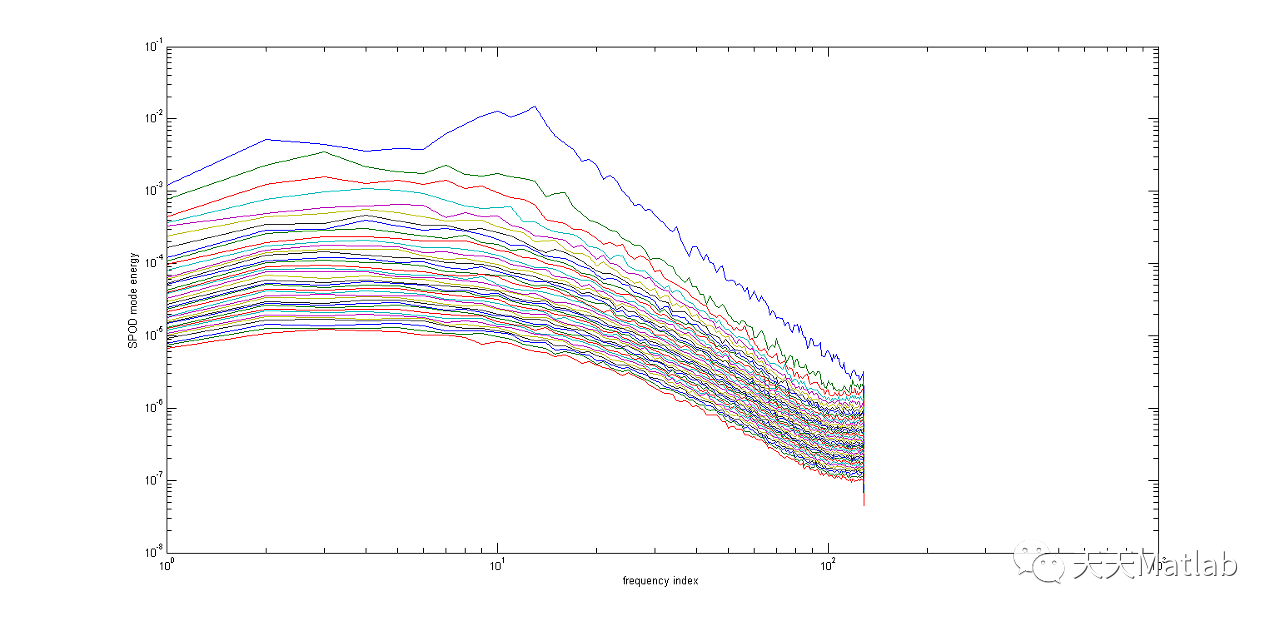
⛄ 运行结果

⛄ 参考文献

[1] A. Nekkanti, O. T. Schmidt, Frequency鈥搕ime analysis, low-rank reconstruction and denoising of turbulent flows using SPOD, Journal of Fluid Mechanics 926, A26, 2021