点赞、关注再看,养成良好习惯
Life is short, U need Python
初学量化投资实战,[快来点我吧]

配对交易策略实战—协整法
基本流程
配对组合 --> 计算价差 --> 决策标准 --> 确定头寸 --> 平仓获利
-
案例描述
- 本案例以上证50股票数据为对象、以协整模型为方法、以Python语言为工具进行配对交易策略的实证分析。在实证分析的过程中,主要借助于 arch 和 statsmodels等第三方库单位根检验和协整检验,进而选取股票对;然后设置决策标准和交易头寸进行回测交易。
-
数据集
- 上证50:sh50_stock_data.csv
-
导入模块
import pandas as pd
import numpy as npimport matplotlib.pyplot as plt
plt.rcParams['font.sans-serif'] = ['SimHei']        # 字体设置
import matplotlib
matplotlib.rcParams['axes.unicode_minus']=False    # 负号显示问题from arch.unitroot import ADF                     # pip install arch
import statsmodels.api as sm
- 导入数据
sh = pd.read_csv('sh50_stock_data.csv',index_col='Trddt')
sh.index = pd.to_datetime(sh.index)
- 形成期:协整检验
# 提取数据
P_zhonghang = sh['601988']   # 中国银行
P_pufa = sh['600000']       # 浦发银行
# 设置形成期
formStart = '2014-01-01'
formEnd = '2015-01-01'P_zhonghang_f = P_zhonghang[formStart:formEnd]
P_pufa_f = P_pufa[formStart:formEnd]
# 形成期:协整关系检验
# 中国银行(A)一阶单整检验
log_P_zhonghang_f = np.log(P_zhonghang_f)adf_zhonghang = ADF(log_P_zhonghang_f)print(adf_zhonghang.summary().as_text())
   Augmented Dickey-Fuller Results
=====================================
Test Statistic                  3.409
P-value                         1.000
Lags                               12
-------------------------------------Trend: Constant
Critical Values: -3.46 (1%), -2.87 (5%), -2.57 (10%)
Null Hypothesis: The process contains a unit root.
Alternative Hypothesis: The process is weakly stationary.
# 形成期:差分后的协整检验
adf_zhonghang_diff = ADF(log_P_zhonghang_f.diff()[1:])print(adf_zhonghang_diff.summary().as_text())
   Augmented Dickey-Fuller Results
=====================================
Test Statistic                 -4.571
P-value                         0.000
Lags                               11
-------------------------------------Trend: Constant
Critical Values: -3.46 (1%), -2.87 (5%), -2.57 (10%)
Null Hypothesis: The process contains a unit root.
Alternative Hypothesis: The process is weakly stationary.
# 形成期:对数序列可视化
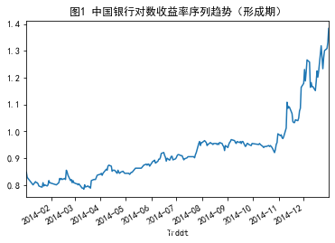
log_P_zhonghang_f.plot()plt.title('图1 中国银行对数收益率序列趋势(形成期)')plt.show()
# 形成期:差分对数序列可视化
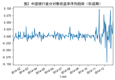
log_P_zhonghang_f.diff()[1:].plot()plt.title('图2 中国银行差分对数收益率序列趋势(形成期)')plt.show()
# 形成期:协整关系检验
# 浦发银行(B)一阶单整检验
log_P_pufa_f = np.log(P_pufa_f)adf_pufa = ADF(log_P_pufa_f)print(adf_pufa.summary().as_text())
   Augmented Dickey-Fuller Results
=====================================
Test Statistic                  2.392
P-value                         0.999
Lags                               12
-------------------------------------Trend: Constant
Critical Values: -3.46 (1%), -2.87 (5%), -2.57 (10%)
Null Hypothesis: The process contains a unit root.
Alternative Hypothesis: The process is weakly stationary.
# 形成期:差分后的协整检验
adf_pufa_diff = ADF(log_P_pufa_f.diff()[1:])print(adf_pufa_diff.summary().as_text())
   Augmented Dickey-Fuller Results
=====================================
Test Statistic                 -3.888
P-value                         0.002
Lags                               11
-------------------------------------Trend: Constant
Critical Values: -3.46 (1%), -2.87 (5%), -2.57 (10%)
Null Hypothesis: The process contains a unit root.
Alternative Hypothesis: The process is weakly stationary.
# 形成期:对数序列可视化
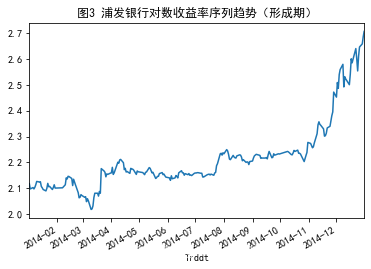
log_P_pufa_f.plot()plt.title('图3 浦发银行对数收益率序列趋势(形成期)')plt.show()
# 形成期:差分对数序列可视化
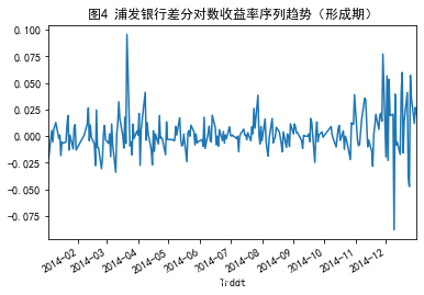
log_P_pufa_f.diff()[1:].plot()plt.title('图4 浦发银行差分对数收益率序列趋势(形成期)')plt.show()
- 形成期:股票对的回归方程(协整模型)
model = sm.OLS(log_P_pufa_f,sm.add_constant(log_P_zhonghang_f))result = model.fit()print(result.summary())
                            OLS Regression Results
==============================================================================
Dep. Variable:                 600000   R-squared:                       0.949
Model:                            OLS   Adj. R-squared:                  0.949
Method:                 Least Squares   F-statistic:                     4560.
Date:                Fri, 20 Nov 2020   Prob (F-statistic):          1.83e-159
Time:                        10:59:05   Log-Likelihood:                 509.57
No. Observations:                 245   AIC:                            -1015.
Df Residuals:                     243   BIC:                            -1008.
Df Model:                           1
Covariance Type:            nonrobust
==============================================================================coef    std err          t      P>|t|      [0.025      0.975]
------------------------------------------------------------------------------
const          1.2269      0.015     83.071      0.000       1.198       1.256
601988         1.0641      0.016     67.531      0.000       1.033       1.095
==============================================================================
Omnibus:                       19.538   Durbin-Watson:                   0.161
Prob(Omnibus):                  0.000   Jarque-Bera (JB):               13.245
Skew:                           0.444   Prob(JB):                      0.00133
Kurtosis:                       2.286   Cond. No.                         15.2
==============================================================================Warnings:
[1] Standard Errors assume that the covariance matrix of the errors is correctly specified.D:\Anaconda3\lib\site-packages\numpy\core\fromnumeric.py:2389: FutureWarning: Method .ptp is deprecated and will be removed in a future version. Use numpy.ptp instead.return ptp(axis=axis, out=out, **kwargs)
# 设置alpha、beta(交易头寸,即投资比例)
alpha = result.params[0]
beta = result.params[1]
- 形成期:残差单位根检验(残差序列为价格差序列)
# 回归方程(形成期)
spread_f = log_P_pufa_f - beta * log_P_zhonghang_f - alphaadfSpread = ADF(spread_f)print(adfSpread.summary().as_text())
   Augmented Dickey-Fuller Results
=====================================
Test Statistic                 -3.193
P-value                         0.020
Lags                                0
-------------------------------------Trend: Constant
Critical Values: -3.46 (1%), -2.87 (5%), -2.57 (10%)
Null Hypothesis: The process contains a unit root.
Alternative Hypothesis: The process is weakly stationary.
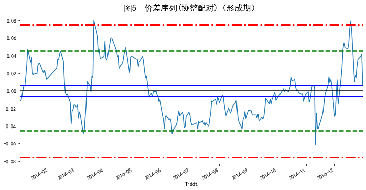
# 计算协整方程中残差序列的均值、方差
mu = np.mean(spread_f)
sd = np.std(spread_f)
- 构造Pair Trading类(封装协整检验)
# 构建类(协整检验)
class PairTrading:# 形成期的协整检验(形成期协整方程残差的ADF检验)def cointegration(self,priceX,priceY):log_priceX = np.log(priceX)log_priceY = np.log(priceY)results = sm.OLS(log_priceY,sm.add_constant(log_priceX)).fit()resid = results.residadfSpread = ADF(resid)if adfSpread.pvalue >= 0.05:print('''交易价格不具有协整关系.P-value of ADF test: %fCoefficients of regression:Intercept: %fBeta: %f''' % (adfSpread.pvalue, results.params[0], results.params[1]))return(None)else:print('''交易价格具有协整关系.P-value of ADF test: %fCoefficients of regression:Intercept: %fBeta: %f''' % (adfSpread.pvalue, results.params[0], results.params[1]))return(results.params[0], results.params[1])# 根据形成期的协整方程系数构造交易期协整方程,进而计算交易期协整残差序列:Co_Spread_Tradedef CointegrationSpread(self,priceX,priceY,formStart,formEnd,tradeStart,tradeEnd):     formX = priceX[formStart:formEnd]formY = priceY[formStart:formEnd]tradeX = priceX[tradeStart:tradeEnd]tradeY = priceY[tradeStart:tradeEnd]coefficients = self.cointegration(formX,formY)if coefficients is None:print('未形成协整关系,无法配对.')else:spread = np.log(tradeY) - coefficients[0] - coefficients[1] * np.log(tradeX)return(spread)# 计算形成期的最优策略阈值:UpperBound 和 LowerBound,作为交易期的策略阈值def Cointegration_calBound(self,priceX,priceY,formStart,formEnd,width):spread = self.CointegrationSpread(priceX,priceY,formStart,formEnd,formStart,formEnd)mu = np.mean(spread)sd = np.std(spread)UpperBound = mu + width * sdLowerBound = mu - width * sdreturn(UpperBound,LowerBound)
# 设定交易期
tradeStart = '2015-01-01'
tradeEnd = '2015-06-30'
# 选取标的
price_zhonghang = sh['601988']
price_pufa = sh['600000']
# 形成期标的价格
price_zhonghang_f = price_zhonghang[formStart:formEnd]
price_pufa_f = price_pufa[formStart:formEnd]
# 类的实例化
pt = PairTrading()         # 调用类PairTrading()
# 协整关系的系数(形成期)
coefficients = pt.cointegration(price_zhonghang_f,price_pufa_f)
交易价格具有协整关系.P-value of ADF test: 0.020415Coefficients of regression:Intercept: 1.226852Beta: 1.064103
# 形成期:价差序列
CoSpreadForm = pt.CointegrationSpread(price_zhonghang,price_pufa,formStart,formEnd,formStart,formEnd)
交易价格具有协整关系.P-value of ADF test: 0.020415Coefficients of regression:Intercept: 1.226852Beta: 1.064103
# 绘制价差序列图(形成期)
plt.figure(figsize=(12,6))CoSpreadForm.plot()plt.title('图5  价差序列(协整配对)(形成期)',loc='center', fontsize=16)plt.axhline(y=mu,color='black')
plt.axhline(y=mu+0.2*sd,color='blue',ls='-',lw=2)
plt.axhline(y=mu-0.2*sd,color='blue',ls='-',lw=2)
plt.axhline(y=mu+1.5*sd,color='green',ls='--',lw=2.5)
plt.axhline(y=mu-1.5*sd,color='green',ls='--',lw=2.5)
plt.axhline(y=mu+2.5*sd,color='red',ls='-.',lw=3)
plt.axhline(y=mu-2.5*sd,color='red',ls='-.',lw=3) plt.show()
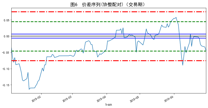
# 交易期:价差序列
CoSpreadTrade = pt.CointegrationSpread(price_zhonghang,price_pufa,formStart,formEnd,tradeStart,tradeEnd)
交易价格具有协整关系.P-value of ADF test: 0.020415Coefficients of regression:Intercept: 1.226852Beta: 1.064103
# 根据形成期协整配对后价差序列得到的阈值
bound = pt.Cointegration_calBound(price_zhonghang,price_pufa,formStart,formEnd,width=1.5)
交易价格具有协整关系.P-value of ADF test: 0.020415Coefficients of regression:Intercept: 1.226852Beta: 1.06410
- 交易期:回测检验
# 提取交易期标的数据
P_zhonghang_t = P_zhonghang[tradeStart:tradeEnd]
P_pufa_t = P_pufa[tradeStart:tradeEnd]
#  计算交易期协整方程的残差序列(价差序列)
CoSpreadTrade = np.log(P_pufa_t) - beta * np.log(P_zhonghang_t) - alpha
# 绘制价格区间图(交易期)
plt.figure(figsize=(12,6))CoSpreadTrade.plot()plt.title('图6  价差序列(协整配对)(交易期)',loc='center', fontsize=16)plt.axhline(y=mu,color='black')
plt.axhline(y=mu+0.2*sd,color='blue',ls='-',lw=2)
plt.axhline(y=mu-0.2*sd,color='blue',ls='-',lw=2)
plt.axhline(y=mu+1.5*sd,color='green',ls='--',lw=2.5)
plt.axhline(y=mu-1.5*sd,color='green',ls='--',lw=2.5)
plt.axhline(y=mu+2.5*sd,color='red',ls='-.',lw=3)
plt.axhline(y=mu-2.5*sd,color='red',ls='-.',lw=3) plt.show()
- 设置策略区间
# 设置触发区间:t_0=0.2; t_1=1.5; t_2=2.5
level = (float('-inf'),mu-2.5*sd,mu-1.5*sd,mu-0.2*sd,mu+0.2*sd,mu+1.5*sd,mu+2.5*sd,float('inf'))
# 把交易期的价差序列按照触发区间标准分类【-3,+3】
prcLevel = pd.cut(CoSpreadTrade,level,labels=False)-3         #剪切函数pd.cut()
pandas.cut: pandas.cut(x, bins, right=True, labels=None,
retbins=False, precision=3, include_lowest=False)参数:
- (1) x,类array对象,且必须为一维,待切割的原形式
- (2) bins, 整数、序列尺度、或间隔索引。如果bins是一个整数,它定义了x宽度范围内的等宽面元数量,但是在这种情况下,x的范围在每个边上被延长1%,以保证包括x的最小值或最大值。如果bin是序列,它定义了允许非均匀bin宽度的bin边缘。在这种情况下没有x的范围的扩展。
- (3) right,布尔值。是否是左开右闭区间
- (4) labels,用作结果箱的标签。必须与结果箱相同长度。如果FALSE,只返回整数指标面元(区间位置,即第几个区间,注意以0位置开始)。
- (5) retbins,布尔值。是否返回面元
- (6) precision,整数。返回面元的小数点几位
- (7) include_lowest,布尔值。第一个区间的左端点是否包含 返回值:
- 若labels为False则返回整数填充的Categorical(分类)或数组或Series(序列)
- 若retbins为True还返回用浮点数填充的N维数组
- 构造交易信号函数
# 构造交易信号函数
def TradeSig(prcLevel):n = len(prcLevel)signal = np.zeros(n)for i in range(1,n):if prcLevel[i-1] == 1 and prcLevel[i] == 2:           # 价差从1区上穿2区,反向建仓signal[i] = -2elif prcLevel[i-1] == 1 and prcLevel[i] == 0:        # 价差从1区下穿0区,平仓signal[i] = 2elif prcLevel[i-1] == 2 and prcLevel[i] == 3:        # 价差从2区上穿3区,即突破3区,平仓signal[i] = 3elif prcLevel[i-1] == -1 and prcLevel[i] == -2:     # 价差从-1区下穿-2区,正向建仓signal[i] = 1elif prcLevel[i-1] == -1 and prcLevel[i] == 0:      # 价差从-1区上穿0区,平仓signal[i] = -1elif prcLevel[i-1] == -2 and prcLevel[i] == -3:     # 价差从-2区下穿-3区,即突破-3区,平仓signal[i] = -3return(signal)
# 设置每个每天的交易信号
signal = TradeSig(prcLevel)
position = [signal[0]]
ns = len(signal)
# 设置每天开仓、平仓指令
for i in range(1,ns):position.append(position[-1])if signal[i] == 1:position[i] = 1                 # 价差从-1区下穿-2区,正向建仓: 买B卖A <------(价差为B-A)elif signal[i] == -2:position[i] = -1               # 价差从1区上穿2区,反向建仓:卖B买A <------(价差为B-A)elif signal[i] == -1 and position[i-1] == 1:position[i] = 0                # 平仓elif signal[i] == 2 and position[i-1] == -1:position[i] = 0               # 平仓elif signal[i] == 3:position[i] = 0              # 平仓elif signal[i] == -3:position[i] = 0             # 平仓
position = pd.Series(position, index=CoSpreadTrade.index)
# 构造交易模拟函数
def TradeSim(priceX,priceY,position):n = len(position)size = 1000                   # 因为浦发银行价格15左右,1000股对应15000,10%—20%保证金即:初始资金cash=1500-3000shareY = size * positionshareX = [(-beta) * shareY[0] * priceY[0] / priceX[0]]    # CoSpreadT = np.log(PBt)-beta*np.log(PAt)-alphacash = [2000]for i in range(1,n):shareX.append(shareX[i-1])cash.append(cash[i-1])if position[i-1] == 0 and position[i] == 1:shareX[i] = (-beta)*shareY[i]*priceY[i]/priceX[i]cash[i] = cash[i-1]-(shareY[i]*priceY[i]+shareX[i]*priceX[i])elif position[i-1] == 0 and position[i] == -1:shareX[i] = (-beta)*shareY[i]*priceY[i]/priceX[i]cash[i] = cash[i-1]-(shareY[i]*priceY[i]+shareX[i]*priceX[i])elif position[i-1] == 1 and position[i] == 0:shareX[i] = 0cash[i] = cash[i-1]+(shareY[i-1]*priceY[i]+shareX[i-1]*priceX[i])elif position[i-1] == -1 and position[i] == 0:shareX[i] = 0cash[i] = cash[i-1]+(shareY[i-1]*priceY[i]+shareX[i-1]*priceX[i])cash = pd.Series(cash,index=position.index)shareY = pd.Series(shareY,index=position.index)shareX = pd.Series(shareX,index=position.index)asset = cash + shareY*priceY + shareX*priceXaccount = pd.DataFrame({'Position':position,'ShareY':shareY,'ShareX':shareX,'Cash':cash,'Asset':asset})return(account)
account = TradeSim(P_zhonghang_t,P_pufa_t,position)
account.iloc[:, [1,2,3,4]].plot(style=['--','--','-',':'], figsize=(16,8))plt.title('图6 配对交易账户(交易期)',loc='center', fontsize=16) plt.show()
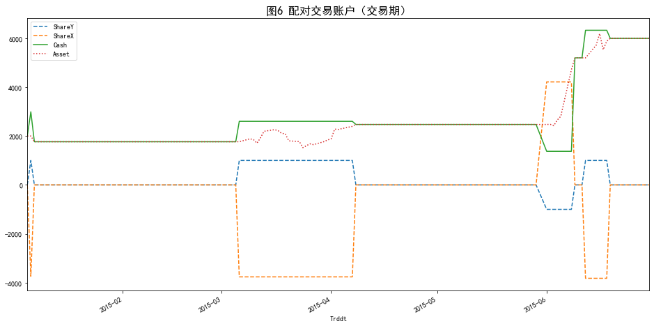
其中,(1)ShareY 可以表示配对仓位(1000倍)(正反向持仓与不持仓);(2)ShareX 表示对应配对仓位(1000倍)(反正向持仓与不持仓);(3)Cash 曲线表示现金的变化,初始现金为2000元;(4)Asset 曲线表示资产的变化。
结论:
-
观察交易仓位曲线图,可以看出自2015年1月1日到2015年6月底期间,配对交易信号触发不多(计4次)。
-
观察现金曲线图,由于开仓可能需要现金,现金曲线有升有降,而第三次平仓之后获利很多,现金曲线大幅上涨,到6月底,现金部位达到了5992.514元。
-
再观察资产曲线图,配对资产整体呈现上升趋势,资产由2000元转变成5992.514元。
-
整体而言,对中国银行和浦发银行两只股票进行配对交易的策略绩效表现不错。
-
构造Back Testing类(封装回测检验)
class BackTesting:     # 构造交易信号函数def TradeSigPosition(self,CoSpreadT,level,k):prcLevel = pd.cut(CoSpreadT,level,labels=False)-kn = len(prcLevel)signal = np.zeros(n)for i in range(1,n):if prcLevel[i-1] == 1 and prcLevel[i] == 2:           # 价差从1区上穿2区,反向建仓signal[i] = -2elif prcLevel[i-1] == 1 and prcLevel[i] == 0:        # 价差从1区下穿0区,平仓signal[i] = 2elif prcLevel[i-1] == 2 and prcLevel[i] == 3:        # 价差从2区上穿3区,即突破3区,平仓signal[i] = 3elif prcLevel[i-1] == -1 and prcLevel[i] == -2:     # 价差从-1区下穿-2区,正向建仓signal[i] = 1elif prcLevel[i-1] == -1 and prcLevel[i] == 0:      # 价差从-1区上穿0区,平仓signal[i] = -1elif prcLevel[i-1] == -2 and prcLevel[i] == -3:     # 价差从-2区下穿-3区,即突破-3区,平仓signal[i] = -3position = [signal[0]]ns = len(signal)# 设置每天开仓、平仓指令for i in range(1,ns):position.append(position[-1])if signal[i] == 1:position[i] = 1                 # 价差从-1区下穿-2区,正向建仓: 买B卖A <------(价差为B-A)elif signal[i] == -2:position[i] = -1               # 价差从1区上穿2区,反向建仓:卖B买A <------(价差为B-A)elif signal[i] == -1 and position[i-1] == 1:position[i] = 0                # 平仓elif signal[i] == 2 and position[i-1] == -1:position[i] = 0               # 平仓elif signal[i] == 3:position[i] = 0              # 平仓elif signal[i] == -3:position[i] = 0             # 平仓position = pd.Series(position, index=CoSpreadT.index)return(position)# 构造交易模拟函数def TradeSim(self,priceX,priceY,position,size,cash):n = len(position)
#         size = 1000                   # 因为浦发银行价格15左右,1000股对应15000,10%—20%保证金即:初始资金cash=1500-3000shareY = size * positionshareX = [(-beta) * shareY[0] * priceY[0] / priceX[0]]    # CoSpreadT = np.log(PBt)-beta*np.log(PAt)-alpha#         cash = [2000]for i in range(1,n):shareX.append(shareX[i-1])cash.append(cash[i-1])if position[i-1] == 0 and position[i] == 1:shareX[i] = (-beta)*shareY[i]*priceY[i]/priceX[i]cash[i] = cash[i-1]-(shareY[i]*priceY[i]+shareX[i]*priceX[i])elif position[i-1] == 0 and position[i] == -1:shareX[i] = (-beta)*shareY[i]*priceY[i]/priceX[i]cash[i] = cash[i-1]-(shareY[i]*priceY[i]+shareX[i]*priceX[i])elif position[i-1] == 1 and position[i] == 0:shareX[i] = 0cash[i] = cash[i-1]+(shareY[i-1]*priceY[i]+shareX[i-1]*priceX[i])elif position[i-1] == -1 and position[i] == 0:shareX[i] = 0cash[i] = cash[i-1]+(shareY[i-1]*priceY[i]+shareX[i-1]*priceX[i])cash = pd.Series(cash,index=position.index)shareY = pd.Series(shareY,index=position.index)shareX = pd.Series(shareX,index=position.index)asset = cash + shareY*priceY + shareX*priceXaccount = pd.DataFrame({'Position':position,'ShareY':shareY,'ShareX':shareX,'Cash':cash,'Asset':asset})return(account)
bt = BackTesting()position = bt.TradeSigPosition(CoSpreadTrade,level,3)account = bt.TradeSim(P_zhonghang_t,P_pufa_t,position,1000,[2000])account.iloc[:, [1,2,3,4]].plot(style=['--','--','-',':'], figsize=(16,8))
plt.title('配对交易账户(交易期)',loc='center', fontsize=16)
plt.show()

参考资料:
- 蔡立耑. 量化投资以Python为工具[M]. 北京:电子工业出版社,2017.
数据下载
- 链接:https://pan.baidu.com/s/1nIFSnTzhTJk2ETh0bJ_SkA
提取码:8gy4
- 写作不易,切勿白剽
- 博友们的点赞和关注就是对博主坚持写作的最大鼓励
- 持续更新,未完待续…