配对交易的步骤

1. 如何挑选进行配对的股票

2. 挑选好股票对以后，如何制定交易策略，开仓点如何设计

3. 开仓是，两只股票如何进行多空仓对比

股票对的选择

1. 行业内匹配

2. 产业链配对

3. 财务管理配对

最小距离法

配对交易需要对股票价格进行标准化处理。假设$P_t^i(t=0,1,2,...,T)$表示股票i在第t天的价格，那么股票i在第t天的单期收益率可以表达为：
$r_t^i=\frac{P_t^i-P_{t-1}^i}{P_{t-1}^i},t=1,2,3,...,T$

用${\hat{p}}_t^i$ 表示股票i在第t天的标准化价格，学界和业界认为${\hat{p}}_t^i$可以有这t天内的累计收益率来计算：
${\hat{p}}_t^i={\prod }_{\tau =1}^t(1+r_{\tau }^i)$

假设有股票X，Y，则我们可以计算二者之间的标准化价差之平方和$SS{D}_{X,Y}$

$SS{D}_{X,Y}={\sum }_{t=1}^T({\hat{p}}_t^X-{\hat{p}}_t^Y{)}^2$

下面使用python计算SSD

import pandas as pd

sh=pd.read_csv('sh50p.csv',index_col='Trddt')

sh.index=pd.to_datetime(sh.index)

sh.head()

	600000	600010	600015	600016	600018	600028	600030	600036	600048	600050	...	601688	601766	601800	601818	601857	601901	601985	601988	601989	601998
Trddt
2010-01-04	9.997	2.260	6.541	4.627	4.775	8.445	17.927	13.174	6.443	6.703	...	-	4.991	-	-	11.284	-	-	3.055	4.591	6.498
2010-01-05	10.072	2.250	6.706	4.708	4.783	8.494	18.804	13.188	6.243	6.937	...	-	4.982	-	-	11.499	-	-	3.090	4.573	6.578
2010-01-06	9.874	2.255	6.461	4.615	4.733	8.311	18.586	12.913	6.237	6.787	...	-	4.947	-	-	11.342	-	-	3.055	4.627	6.393
2010-01-07	9.652	2.201	6.328	4.493	4.602	8.091	18.133	12.578	6.240	6.590	...	-	4.875	-	-	11.267	-	-	2.998	4.573	6.176
2010-01-08	9.761	2.211	6.370	4.539	4.618	8.005	18.483	12.578	6.322	6.674	...	-	4.902	-	-	11.135	-	-	3.012	4.525	6.232

5 rows × 50 columns

# 定义配对形成期
formStart='2014-01-01'
formEnd='2015-01-01'

# 形成期数据
shform=sh[formStart:formEnd]

shform.head(2)

	600000	600010	600015	600016	600018	600028	600030	600036	600048	600050	...	601688	601766	601800	601818	601857	601901	601985	601988	601989	601998
Trddt
2014-01-02	8.307	2.360	6.371	6.183	5.031	4.117	12.288	9.719	5.156	3.146	...	8.534	4.869	3.781	2.383	7.245	5.91	-	2.333	5.617	3.634
2014-01-03	8.138	2.594	6.187	6.087	4.906	4.043	11.937	9.520	5.112	3.088	...	8.293	4.791	3.725	2.356	7.217	5.91	-	2.289	5.517	3.578

2 rows × 50 columns

# 提取中国银行 601988 的收盘价数据
PAf=shform['601988']

# 提取浦发银行 600000 的收盘价数据
PBf = shform['600000']

#合并两只股票
pairf=pd.concat([PAf,PBf],axis=1)

len(pairf)

245

import numpy as np

# 构造标准化价格之差平方累计SSD函数
def SSD(priceX,priceY):if priceX is None or priceY is None:print('缺少价格序列')returnX = (priceX-priceX.shift(1))/priceX.shift(1)[1:]returnY = (priceY-priceY.shift(1))/priceY.shift(1)[1:]standardX=(returnX+1).cumprod()standardY=(returnY+1).cumprod()SSD = np.sum((standardX-standardY)**2)return SSD

dis=SSD(PAf,PBf)

dis

0.47481704588389073

SSD_rst=[]
for i in shform.columns:for j in shform.columns:if i==j:continue;A=shform[i]B=shform[j]try:num=SSD(A,B)except:continue# print(i,j,num)try:lst=[i,j,num]except:continueSSD_rst.append(lst)

SSDdf=pd.DataFrame(SSD_rst)

SSDdf.head()

	0	1	2
0	600000	600010	7.366730
1	600000	600015	0.668806
2	600000	600016	2.563524
3	600000	600018	7.823916
4	600000	600028	3.976679

SSDdf.sort_values(by=2)

	0	1	2
102	600015	601166	0.245662
977	601166	600015	0.245662
1435	601857	601398	0.329987
1244	601398	601857	0.329987
387	600050	601988	0.422743
1452	601988	600050	0.422743
984	601166	600050	0.446014
375	600050	601166	0.446014
1443	601988	600000	0.474817
36	600000	601988	0.474817
300	600036	601318	0.485505
1099	601318	600036	0.485505
1445	601988	600015	0.519690
114	600015	601988	0.519690
982	601166	600036	0.533362
297	600036	601166	0.533362
353	600050	600015	0.545751
86	600015	600050	0.545751
1011	601166	601988	0.546044
1468	601988	601166	0.546044
1002	601166	601318	0.568370
1117	601318	601166	0.568370
303	600036	601398	0.653760
1216	601398	600036	0.653760
948	601088	600111	0.656164
491	600111	601088	0.656164
78	600015	600000	0.668806
1	600000	600015	0.668806
381	600050	601398	0.704233
1218	601398	600050	0.704233
...	...	...	...
479	600111	600109	64.595128
440	600109	600111	64.595128
1434	601857	601390	65.941405
1205	601390	601857	65.941405
947	601088	600109	67.396051
452	600109	601088	67.396051
1186	601390	600585	71.932721
653	600585	601390	71.932721
1204	601390	601766	72.876730
1395	601766	601390	72.876730
1174	601390	600018	73.037316
185	600018	601390	73.037316
689	600637	601186	75.475072
1070	601186	600637	75.475072
674	600637	600109	78.702164
445	600109	600637	78.702164
965	601088	601390	79.636906
1194	601390	601088	79.636906
1182	601390	600111	81.322417
497	600111	601390	81.322417
809	600887	601390	82.309679
1190	601390	600887	82.309679
1067	601186	600518	87.971590
572	600518	601186	87.971590
442	600109	600518	96.995893
557	600518	600109	96.995893
692	600637	601390	97.687461
1187	601390	600637	97.687461
1184	601390	600518	111.693514
575	600518	601390	111.693514

1560 rows × 3 columns

协整模型

协整模型指如果X股票的对数价格是非平稳时间序列，且对数价格的差分序列是平稳的，责成X股票的对数价格是一阶单整序列。
又$$\begin{gathered} log(P_t^X)-log(P_{t-1}^X)=log(\frac{P_t^X}{P_{t-1}^X}) \\ =log(1+r_t^X) \\ =r_t^X \end{gathered}$$

下面计算中国银行和浦发银行是否是一阶单整序列

from arch.unitroot import ADF

import numpy as np

PAf.head()

Trddt
2014-01-02    2.333
2014-01-03    2.289
2014-01-06    2.262
2014-01-07    2.253
2014-01-08    2.244
Name: 601988, dtype: float64

PAflog=np.log(PAf)

adfA=ADF(PAflog)

print(adfA.summary().as_text())

   Augmented Dickey-Fuller Results   
=====================================
Test Statistic                  3.409
P-value                         1.000
Lags                               12
-------------------------------------Trend: Constant
Critical Values: -3.46 (1%), -2.87 (5%), -2.57 (10%)
Null Hypothesis: The process contains a unit root.
Alternative Hypothesis: The process is weakly stationary.

统计量较大，我们接受原假设，原序列存在单位根，所以中国银行的收盘价的对数序列是非平稳序列

#对数差分
retA=PAflog.diff()[1:]

retA.head()

Trddt
2014-01-03   -0.019040
2014-01-06   -0.011866
2014-01-07   -0.003987
2014-01-08   -0.004003
2014-01-09   -0.004019
Name: 601988, dtype: float64

adfretA=ADF(retA)

print(adfretA.summary().as_text())

   Augmented Dickey-Fuller Results   
=====================================
Test Statistic                 -4.571
P-value                         0.000
Lags                               11
-------------------------------------Trend: Constant
Critical Values: -3.46 (1%), -2.87 (5%), -2.57 (10%)
Null Hypothesis: The process contains a unit root.
Alternative Hypothesis: The process is weakly stationary.

统计量较小，所以我们拒绝原假设，对数差分序列没有单位根，所以中国银行的对数差分序列是平稳序列

由此说明中国银行的对数价格序列是一阶单整序列

# 对浦发银行进行检验
PBflog=np.log(PBf)

adfB=ADF(PBflog)

print(adfB.summary().as_text())

   Augmented Dickey-Fuller Results   
=====================================
Test Statistic                  2.392
P-value                         0.999
Lags                               12
-------------------------------------Trend: Constant
Critical Values: -3.46 (1%), -2.87 (5%), -2.57 (10%)
Null Hypothesis: The process contains a unit root.
Alternative Hypothesis: The process is weakly stationary.

统计量较大，我们接受原假设，原序列存在单位根，所以浦发银行的收盘价的对数序列是非平稳序列

#对数差分序列
retB = PBflog.diff()[1:]

adfretB=ADF(retB)

print(adfretB.summary().as_text())

   Augmented Dickey-Fuller Results   
=====================================
Test Statistic                 -3.888
P-value                         0.002
Lags                               11
-------------------------------------Trend: Constant
Critical Values: -3.46 (1%), -2.87 (5%), -2.57 (10%)
Null Hypothesis: The process contains a unit root.
Alternative Hypothesis: The process is weakly stationary.

统计量较小，所以拒绝原假设，不存在单位根，所以浦发银行的对数差分序列是平稳序列

由此说明浦发银行的对数序列是一阶单整序列

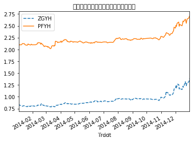
#绘制对数时序图
import matplotlib.pyplot as plt

PAflog.plot(label='ZGYH',style='--')
PBflog.plot(label='PFYH',style='-')
plt.legend(loc='upper left')
plt.title("中国银行和浦发银行的对数价格时序图")

Text(0.5, 1.0, '中国银行和浦发银行的对数价格时序图')

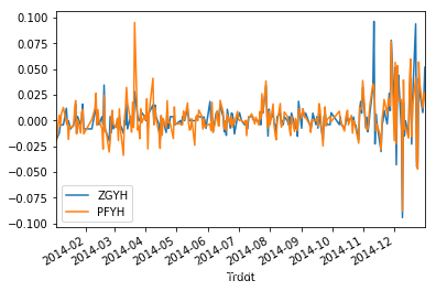
retA.plot(label='ZGYH')
retB.plot(label='PFYH')
plt.legend(loc='lower left')

<matplotlib.legend.Legend at 0x1c238d0eb8>

检验两个对数序列的协整性

方式是对两个序列进行线性拟合，对残差进行检验，如果残差序列是平稳的，说明两个对数序列具有协整性

import statsmodels.api as sm

model=sm.OLS(PBflog,sm.add_constant(PAflog))

/Users/yaochenli/anaconda3/lib/python3.7/site-packages/numpy/core/fromnumeric.py:2389: FutureWarning: Method .ptp is deprecated and will be removed in a future version. Use numpy.ptp instead.return ptp(axis=axis, out=out, **kwargs)

results=model.fit()

print(results.summary())

                            OLS Regression Results                            
==============================================================================
Dep. Variable:                 600000   R-squared:                       0.949
Model:                            OLS   Adj. R-squared:                  0.949
Method:                 Least Squares   F-statistic:                     4560.
Date:                Fri, 23 Aug 2019   Prob (F-statistic):          1.83e-159
Time:                        17:40:05   Log-Likelihood:                 509.57
No. Observations:                 245   AIC:                            -1015.
Df Residuals:                     243   BIC:                            -1008.
Df Model:                           1                                         
Covariance Type:            nonrobust                                         
==============================================================================coef    std err          t      P>|t|      [0.025      0.975]
------------------------------------------------------------------------------
const          1.2269      0.015     83.071      0.000       1.198       1.256
601988         1.0641      0.016     67.531      0.000       1.033       1.095
==============================================================================
Omnibus:                       19.538   Durbin-Watson:                   0.161
Prob(Omnibus):                  0.000   Jarque-Bera (JB):               13.245
Skew:                           0.444   Prob(JB):                      0.00133
Kurtosis:                       2.286   Cond. No.                         15.2
==============================================================================Warnings:
[1] Standard Errors assume that the covariance matrix of the errors is correctly specified.

结果比较显著

对残差进行平稳性检验

#提取回归截距
alpha=results.params[0]

beta =results.params[1]

spread=PBflog-beta*PAflog-alpha

spread.head()

Trddt
2014-01-02   -0.011214
2014-01-03   -0.011507
2014-01-06    0.006511
2014-01-07    0.005361
2014-01-08    0.016112
dtype: float64

spread.plot()

<matplotlib.axes._subplots.AxesSubplot at 0x1c23a44470>

# 价差序列单位根检验
# 因为残差的均值是0，所以trend设为nc
adfSpread=ADF(spread,trend='nc')

print(adfSpread.summary().as_text())

   Augmented Dickey-Fuller Results   
=====================================
Test Statistic                 -3.199
P-value                         0.001
Lags                                0
-------------------------------------Trend: No Trend
Critical Values: -2.57 (1%), -1.94 (5%), -1.62 (10%)
Null Hypothesis: The process contains a unit root.
Alternative Hypothesis: The process is weakly stationary.

统计量较小，所以拒绝原假设，认为残差是平稳的

配对交易策略的制定

最小距离法

计算形成期内标准化的价格序列差${\hat{P}}_t^X-{\hat{P}}_t^Y$的平均值$\mu$和标准差$\sigma$，设定交易信号出发点为$\mu +-2\sigma$交易期为6个月。由于浦发银行和中国银行为银行业股票，价格比较稳定，因此我们设定交易期内价差超过$\mu +-1.2\sigma$时触发交易信号。

#最短距离法交易策略
#中国银行的标准化价格
standardA=(1+retA).cumprod()

#浦发银行的标准化价格
standardB=(1+retB).cumprod()

#标准价差
SSD_pair=standardB-standardA

SSD_pair.head()

Trddt
2014-01-03   -0.001514
2014-01-06    0.015407
2014-01-07    0.013962
2014-01-08    0.024184
2014-01-09    0.037629
dtype: float64

meanSSD_pair = np.mean(SSD_pair)

sdSSD_pair=np.std(SSD_pair)

thresholdUP=meanSSD_pair+1.2*sdSSD_pair

thresholdDOWN=meanSSD_pair-1.2*sdSSD_pair

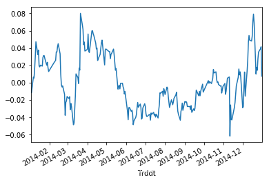
SSD_pair.plot()
plt.axhline(y=meanSSD_pair,color='black')
plt.axhline(y=thresholdUP,color='blue')
plt.axhline(y=thresholdDOWN,color='red')

<matplotlib.lines.Line2D at 0x1c24027860>

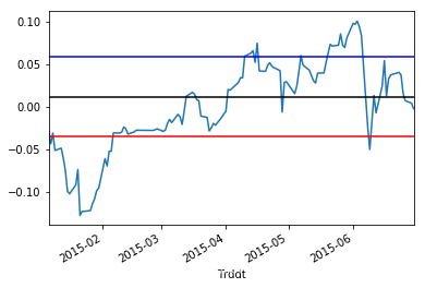
在交易期当价差上穿阀值的时候反向开仓，回归平均线左右的时候平仓，当价差下穿阀值线的时候正向开仓，在价差回归平均线左右的时候平仓。

#交易期
tradStart='2015-01-01'

tradEnd='2015-06-30'

PAt=sh.loc[tradStart:tradEnd,'601988']
PBt=sh.loc[tradStart:tradEnd,'600000']

def spreadCal(x,y):retx=(x-x.shift(1))/x.shift(1)[1:]rety=(y-y.shift(1))/y.shift(1)[1:]standardX=(1+retx).cumprod()standardY=(1+rety).cumprod()spread=standardY-standardXreturn spread

TradSpread=spreadCal(PAt,PBt).dropna()

TradSpread.describe()

count    118.000000
mean       0.001064
std        0.054323
min       -0.127050
25%       -0.028249
50%        0.005682
75%        0.041375
max        0.100249
dtype: float64

TradSpread.plot()
plt.axhline(y=meanSSD_pair,color='black')
plt.axhline(y=thresholdUP,color='blue')
plt.axhline(y=thresholdDOWN,color='red')

<matplotlib.lines.Line2D at 0x1c240f9a58>

协整模型

构建PairTrading类

import re
import pandas as pd
import numpy as np
from arch.unitroot import ADF
import statsmodels.api as sm
class PairTrading:#计算两个股票之间的距离def SSD(self,priceX,priceY):if priceX is None or priceY is None:print('缺少价格序列')returnreturnX=(priceX-priceX.shift(1))/priceX.shift(1)[1:]returnY=(priceY-priceY.shift(1))/priceY.shift(1)[1:]standardX=(1+returnX).cumprod()standardY=(1+returnY).cumprod()SSD=np.sum((standardY-standardX)**2)return SSD#计算标准价差序列def SSDSpread(self,priceX,priceY):if priceX is None or priceY is None:print('缺少价格徐磊')returnreturnX=(priceX-priceX.shift(1))/priceX.shift(1)[1:]returnY=(priceY-priceY.shift(1))/priceY.shift(1)[1:]standardX=(1+returnX).cumprod()standardY=(1+returnY).cumprod()spread=standardY-standardXreturn spread#判断是否是协整序列，并返回协整序列的线性回归参数def cointegration(self,priceX,priceY):if priceX is None or priceY is None:print('缺少价格序列.')priceX=np.log(priceX)priceY=np.log(priceY)results=sm.OLS(priceY,sm.add_constant(priceX)).fit()resid=results.residadfSpread=ADF(resid)if adfSpread.pvalue>=0.05:print('''交易价格不具有协整关系.P-value of ADF test: %fCoefficients of regression:Intercept: %fBeta: %f''' % (adfSpread.pvalue, results.params[0], results.params[1]))return(None)else:print('''交易价格具有协整关系.P-value of ADF test: %fCoefficients of regression:Intercept: %fBeta: %f''' % (adfSpread.pvalue, results.params[0], results.params[1]))return(results.params[0], results.params[1])#计算协整序列差def CointegrationSpread(self,priceX,priceY,formPeriod,tradePeriod):if priceX is None or priceY is None:print('缺少价格序列.')if not (re.fullmatch('\d{4}-\d{2}-\d{2}:\d{4}-\d{2}-\d{2}',formPeriod)or re.fullmatch('\d{4}-\d{2}-\d{2}:\d{4}-\d{2}-\d{2}',tradePeriod)):print('形成期或交易期格式错误.')formX=priceX[formPeriod.split(':')[0]:formPeriod.split(':')[1]]formY=priceY[formPeriod.split(':')[0]:formPeriod.split(':')[1]]coefficients=self.cointegration(formX,formY)if coefficients is None:print('未形成协整关系,无法配对.')else:spread=(np.log(priceY[tradePeriod.split(':')[0]:tradePeriod.split(':')[1]])-coefficients[0]-coefficients[1]*np.log(priceX[tradePeriod.split(':')[0]:tradePeriod.split(':')[1]]))return(spread)#计算边界def calBound(self,priceX,priceY,method,formPeriod,width=1.5):if not (re.fullmatch('\d{4}-\d{2}-\d{2}:\d{4}-\d{2}-\d{2}',formPeriod)or re.fullmatch('\d{4}-\d{2}-\d{2}:\d{4}-\d{2}-\d{2}',tradePeriod)):print('形成期或交易期格式错误.')if method=='SSD':spread=self.SSDSpread(priceX[formPeriod.split(':')[0]:formPeriod.split(':')[1]],priceY[formPeriod.split(':')[0]:formPeriod.split(':')[1]])            mu=np.mean(spread)sd=np.std(spread)UpperBound=mu+width*sdLowerBound=mu-width*sdreturn(UpperBound,LowerBound)elif method=='Cointegration':spread=self.CointegrationSpread(priceX,priceY,formPeriod,formPeriod)mu=np.mean(spread)sd=np.std(spread)UpperBound=mu+width*sdLowerBound=mu-width*sdreturn(UpperBound,LowerBound)else:print('不存在该方法. 请选择"SSD"或是"Cointegration".')

formPeriod='2014-01-01:2015-01-01'
tradePeriod='2015-01-01:2015-06-30'

priceA=sh['601988']
priceB=sh['600000']
priceAf=priceA[formPeriod.split(':')[0]:formPeriod.split(':')[1]]
priceBf=priceB[formPeriod.split(':')[0]:formPeriod.split(':')[1]]
priceAt=priceA[tradePeriod.split(':')[0]:tradePeriod.split(':')[1]]
priceBt=priceB[tradePeriod.split(':')[0]:tradePeriod.split(':')[1]]

pt=PairTrading()
SSD=pt.SSD(priceAf,priceBf)
SSD

0.47481704588389073

SSDspread=pt.SSDSpread(priceAf,priceBf)
SSDspread.describe()
SSDspread.head()

Trddt
2014-01-02         NaN
2014-01-03   -0.001484
2014-01-06    0.015385
2014-01-07    0.013946
2014-01-08    0.024184
dtype: float64

coefficients=pt.cointegration(priceAf,priceBf)
coefficients

交易价格具有协整关系.P-value of ADF test: 0.020415Coefficients of regression:Intercept: 1.226852Beta: 1.064103(1.2268515742404387, 1.0641034525888144)

CoSpreadF=pt.CointegrationSpread(priceA,priceB,formPeriod,formPeriod)
CoSpreadF.head()

交易价格具有协整关系.P-value of ADF test: 0.020415Coefficients of regression:Intercept: 1.226852Beta: 1.064103Trddt
2014-01-02   -0.011214
2014-01-03   -0.011507
2014-01-06    0.006511
2014-01-07    0.005361
2014-01-08    0.016112
dtype: float64

CoSpreadTr=pt.CointegrationSpread(priceA,priceB,formPeriod,tradePeriod)
CoSpreadTr.describe()

交易价格具有协整关系.P-value of ADF test: 0.020415Coefficients of regression:Intercept: 1.226852Beta: 1.064103count    119.000000
mean      -0.037295
std        0.052204
min       -0.163903
25%       -0.063038
50%       -0.033336
75%        0.000503
max        0.057989
dtype: float64

bound=pt.calBound(priceA,priceB,'Cointegration',formPeriod,width=1.2)
bound

交易价格具有协整关系.P-value of ADF test: 0.020415Coefficients of regression:Intercept: 1.226852Beta: 1.064103(0.03627938704534019, -0.03627938704533997)

#配对交易实测
#提取形成期数据
formStart='2014-01-01'
formEnd='2015-01-01'
PA=sh['601988']
PB=sh['600000']PAf=PA[formStart:formEnd]
PBf=PB[formStart:formEnd]

#形成期协整关系检验
#一阶单整检验
log_PAf=np.log(PAf)
adfA=ADF(log_PAf)
print(adfA.summary().as_text())
adfAd=ADF(log_PAf.diff()[1:])
print(adfAd.summary().as_text())

   Augmented Dickey-Fuller Results   
=====================================
Test Statistic                  3.409
P-value                         1.000
Lags                               12
-------------------------------------Trend: Constant
Critical Values: -3.46 (1%), -2.87 (5%), -2.57 (10%)
Null Hypothesis: The process contains a unit root.
Alternative Hypothesis: The process is weakly stationary.Augmented Dickey-Fuller Results   
=====================================
Test Statistic                 -4.571
P-value                         0.000
Lags                               11
-------------------------------------Trend: Constant
Critical Values: -3.46 (1%), -2.87 (5%), -2.57 (10%)
Null Hypothesis: The process contains a unit root.
Alternative Hypothesis: The process is weakly stationary.

log_PBf=np.log(PBf)
adfB=ADF(log_PBf)
print(adfB.summary().as_text())
adfBd=ADF(log_PBf.diff()[1:])
print(adfBd.summary().as_text())

   Augmented Dickey-Fuller Results   
=====================================
Test Statistic                  2.392
P-value                         0.999
Lags                               12
-------------------------------------Trend: Constant
Critical Values: -3.46 (1%), -2.87 (5%), -2.57 (10%)
Null Hypothesis: The process contains a unit root.
Alternative Hypothesis: The process is weakly stationary.Augmented Dickey-Fuller Results   
=====================================
Test Statistic                 -3.888
P-value                         0.002
Lags                               11
-------------------------------------Trend: Constant
Critical Values: -3.46 (1%), -2.87 (5%), -2.57 (10%)
Null Hypothesis: The process contains a unit root.
Alternative Hypothesis: The process is weakly stationary.

#协整关系检验
model=sm.OLS(log_PBf,sm.add_constant(log_PAf)).fit()
model.summary() 

OLS Regression Results

Dep. Variable:	600000	R-squared:	0.949
Model:	OLS	Adj. R-squared:	0.949
Method:	Least Squares	F-statistic:	4560.
Date:	Fri, 23 Aug 2019	Prob (F-statistic):	1.83e-159
Time:	17:43:03	Log-Likelihood:	509.57
No. Observations:	245	AIC:	-1015.
Df Residuals:	243	BIC:	-1008.
Df Model:	1
Covariance Type:	nonrobust

	coef	std err	t	P>|t|	[0.025	0.975]
const	1.2269	0.015	83.071	0.000	1.198	1.256
601988	1.0641	0.016	67.531	0.000	1.033	1.095

Omnibus:	19.538	Durbin-Watson:	0.161
Prob(Omnibus):	0.000	Jarque-Bera (JB):	13.245
Skew:	0.444	Prob(JB):	0.00133
Kurtosis:	2.286	Cond. No.	15.2

Warnings:
[1] Standard Errors assume that the covariance matrix of the errors is correctly specified.

alpha=model.params[0]
alpha 

1.2268515742404387

beta=model.params[1]
beta 

1.0641034525888144

#残差单位根检验
spreadf=log_PBf-beta*log_PAf-alpha
adfSpread=ADF(spreadf)

print(adfSpread.summary().as_text())

   Augmented Dickey-Fuller Results   
=====================================
Test Statistic                 -3.193
P-value                         0.020
Lags                                0
-------------------------------------Trend: Constant
Critical Values: -3.46 (1%), -2.87 (5%), -2.57 (10%)
Null Hypothesis: The process contains a unit root.
Alternative Hypothesis: The process is weakly stationary.

mu=np.mean(spreadf)
sd=np.std(spreadf)

#设定交易期tradeStart='2015-01-01'
tradeEnd='2015-06-30'

PAt=PA[tradeStart:tradeEnd]
PBt=PB[tradeStart:tradeEnd]

CoSpreadT=np.log(PBt)-beta*np.log(PAt)-alpha

CoSpreadT.describe()

count    119.000000
mean      -0.037295
std        0.052204
min       -0.163903
25%       -0.063038
50%       -0.033336
75%        0.000503
max        0.057989
dtype: float64

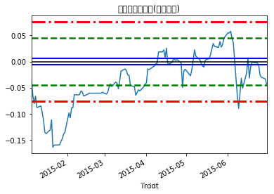
CoSpreadT.plot()
plt.title('交易期价差序列(协整配对)')
plt.axhline(y=mu,color='black')
plt.axhline(y=mu+0.2*sd,color='blue',ls='-',lw=2)
plt.axhline(y=mu-0.2*sd,color='blue',ls='-',lw=2)
plt.axhline(y=mu+1.5*sd,color='green',ls='--',lw=2.5)
plt.axhline(y=mu-1.5*sd,color='green',ls='--',lw=2.5)
plt.axhline(y=mu+2.5*sd,color='red',ls='-.',lw=3) 
plt.axhline(y=mu-2.5*sd,color='red',ls='-.',lw=3)

<matplotlib.lines.Line2D at 0x1c2431b470>

level=(float('-inf'),mu-2.5*sd,mu-1.5*sd,mu-0.2*sd,mu+0.2*sd,mu+1.5*sd,mu+2.5*sd,float('inf'))

prcLevel=pd.cut(CoSpreadT,level,labels=False)-3

prcLevel.head()

Trddt
2015-01-05   -1
2015-01-06   -2
2015-01-07   -3
2015-01-08   -2
2015-01-09   -3
dtype: int64

def TradeSig(prcLevel):n=len(prcLevel)signal=np.zeros(n)for i in range(1,n):#反向建仓if prcLevel[i-1]==1 and prcLevel[i]==2:signal[i]=-2#反向平仓elif prcLevel[i-1]==1 and prcLevel[i]==0:signal[i]=2#强制平仓elif prcLevel[i-1]==2 and prcLevel[i]==3:signal[i]=3#正向建仓elif prcLevel[i-1]==-1 and prcLevel[i]==-2:signal[i]=1#正向平仓elif prcLevel[i-1]==-1 and prcLevel[i]==0:signal[i]=-1#强制平仓elif prcLevel[i-1]==-2 and prcLevel[i]==-3:signal[i]=-3return(signal)

signal=TradeSig(prcLevel)

position=[signal[0]]
ns=len(signal)

for i in range(1,ns):position.append(position[-1])#正向建仓if signal[i]==1:position[i]=1#反向建仓elif signal[i]==-2:position[i]=-1#正向平仓elif signal[i]==-1 and position[i-1]==1:position[i]=0#反向平仓elif signal[i]==2 and position[i-1]==-1:position[i]=0#强制平仓elif signal[i]==3:position[i]=0elif signal[i]==-3:position[i]=0

position=pd.Series(position,index=CoSpreadT.index)

position.tail()

Trddt
2015-06-24    0.0
2015-06-25    0.0
2015-06-26    0.0
2015-06-29    0.0
2015-06-30    0.0
dtype: float64

def TradeSim(priceX,priceY,position):n=len(position)size=1000shareY=size*positionshareX=[(-beta)*shareY[0]*priceY[0]/priceX[0]]cash=[2000]for i in range(1,n):shareX.append(shareX[i-1])cash.append(cash[i-1])if position[i-1]==0 and position[i]==1:shareX[i]=(-beta)*shareY[i]*priceY[i]/priceX[i]cash[i]=cash[i-1]-(shareY[i]*priceY[i]+shareX[i]*priceX[i])elif position[i-1]==0 and position[i]==-1:shareX[i]=(-beta)*shareY[i]*priceY[i]/priceX[i]cash[i]=cash[i-1]-(shareY[i]*priceY[i]+shareX[i]*priceX[i])elif position[i-1]==1 and position[i]==0:shareX[i]=0cash[i]=cash[i-1]+(shareY[i-1]*priceY[i]+shareX[i-1]*priceX[i])elif position[i-1]==-1 and position[i]==0:shareX[i]=0cash[i]=cash[i-1]+(shareY[i-1]*priceY[i]+shareX[i-1]*priceX[i])cash = pd.Series(cash,index=position.index)shareY=pd.Series(shareY,index=position.index)shareX=pd.Series(shareX,index=position.index)asset=cash+shareY*priceY+shareX*priceXaccount=pd.DataFrame({'Position':position,'ShareY':shareY,'ShareX':shareX,'Cash':cash,'Asset':asset})return(account)

account=TradeSim(PAt,PBt,position)
account.tail() 

	Position	ShareY	ShareX	Cash	Asset
Trddt
2015-06-24	0.0	0.0	0.0	5992.514	5992.514
2015-06-25	0.0	0.0	0.0	5992.514	5992.514
2015-06-26	0.0	0.0	0.0	5992.514	5992.514
2015-06-29	0.0	0.0	0.0	5992.514	5992.514
2015-06-30	0.0	0.0	0.0	5992.514	5992.514

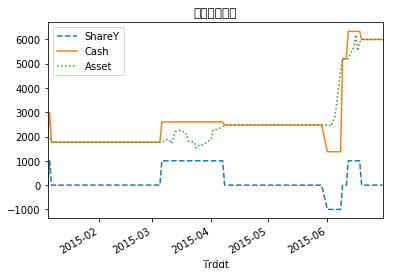
account.iloc[:,[1,3,4]].plot(style=['--','-',':'])
plt.title('配对交易账户') 

Text(0.5, 1.0, '配对交易账户')