写在前面
之前做了一个2022年Mathorcup数学建模挑战赛C题的比赛心得,上一篇文章主要讲了A*算法的改进以及A*算法如何在C题的第3问的应用。本文主要介绍C题的第2问,即三种泊车模型如何建立,因此部分并非我写,在比赛期间,我主要攻克的是第3问,因此,写这篇文章也花了我不少心思,重新看代码,跑代码,尽可能详细地讲清楚泊车模型地建立,希望能够帮到有需要的同学。
题目
先来看问题:
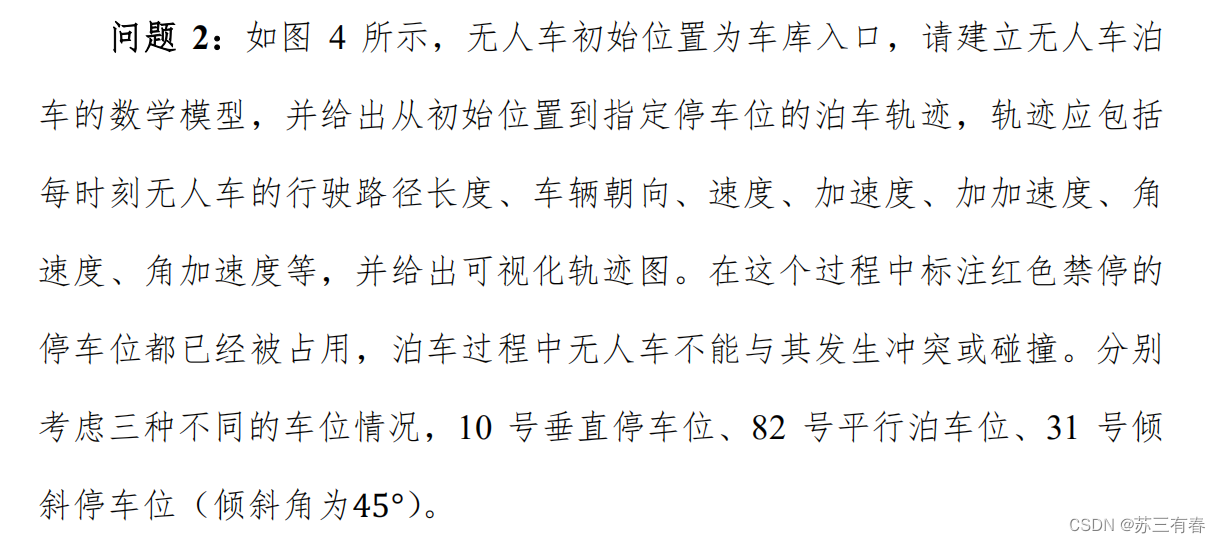
图4如下:

根据题目要求,我们要做出车辆从初始位置到10号垂直停车位,82号平行停车位以及31号倾斜停车位的轨迹图,加速度,加加速度,路径长度....等等。
在本文中,我们不考虑各种物理量的求解以及关于最小转弯半径等问题,我们仅考虑最重要的部分,也就是车辆到达停车位附近后,该如何停进停车位。
问题分析
在该问题中,我们要实现车辆停进垂直停车位,水平停车位,倾斜停车位,也就是说,我们要建立三种不同的泊车模型。
首先,我们先对数据做了预处理,即我们假设,每种停车方式,都能通过把方向盘打死(方向盘打死后就可以达到最小转弯半径,最容易停进停车位),一次性倒车入库。
一次性倒车入库的意思是:车辆只需要后退,不需要前进调整位置,在后退过程中可以更改方向盘方向。
我们通过查找文献,计算车辆的最小转弯半径以及最小通过圆,为什么要计算这两个值呢?
因为我们要粗略计算,一次性倒车入库时,我们会不会碰撞到边界,即车身转弯时所画出的环(这个环就是车身在转弯时所经过的地方,这个环内不允许有任何东西,有的话就会碰撞到)会不会与边界相交。
关于最小转弯半径的原理以及计算公式,最小通过圆概念的博客如下:
最小转弯半径的计算,最小通过圆,含图片
了解了最小转弯半径以及最小通过圆后,我们可以继续:
例如:
假设黑线是车辆方向盘打死的情况下,计算得到的最外层侧转弯半径以及最内侧转弯半径,则由这两个半径所构成的环已经碰撞到边界了,因此此时车辆是无法一次性倒车入库的。
(我们这里用最终状态来反推初始状态)
具体的计算是:
- 先计算最小转弯半径
- 因为车辆转弯时,车身处处作同心圆的转弯,因此,车辆转弯时,转弯圆心固定,车身不同部分的转弯半径不同,通过最小转弯半径,计算最内侧的圆的半径以及最外侧的圆的半径
- 现已知最内侧圆的半径,最外侧圆的半径,建立坐标系,原点选取在一个比较好计算的位置,这个随你
- 建立好坐标系,将边界画出,用函数表示,因为边界皆为竖或横,用y=c,x=c即可
- 不断调整圆心,看是否存在一个圆心,使得最外侧圆与最内侧圆所构成的环中不经过边界
很遗憾的是,通过计算,在三种泊车模型中,仅有垂直泊车是可以一次性倒入库的,平行泊车与倾斜泊车是无法一次性倒入库的,因此,平行泊车与倾斜泊车的复杂程度要远远高于垂直泊车。
因此我们必须想另一种方法来建立泊车模型:既然一次性倒车不行,那么只能多次,反复前进后退来改变车辆自身位置,慢慢将车辆挪进停车位。
我们同样用反溯法,从车辆已经停好的状态反推初始状态,将车辆从停车位中挪出即可。
接下来,我们仅以水平泊车模型作为例子,倾斜泊车模型与水平泊车相似,将碰撞边界以及车辆初始位置改动即可。垂直泊车模型不需要用该模型,只要确定转动圆心以及转动半径即可。
因此,同样以上图的水平停车位为例,其遍历步骤为:
- 车辆运动矢量向左,开始前进
- 若碰到边界则停止运动,若无则继续前进
- 车辆运动矢量向右,开始后退
- 如碰到边界则停止运动,若无则继续后退
- 在坐标轴中,以车辆右侧做一条直线,若右侧边界最突出点在直线下方,则退出循环,若在直线上方,则继续上述循环。
模型建立
给出下面模型所需要的各种全局变量:
addpath lib; R=4.97;
global car_Len car_Wid car_Weel_Den car_Cen_Cen; % 车辆参数
global car_alpha car_oil_ddt car_speed_dt car_speed_ddt car_FXP_speed bump_den bump_speed park_forward_Speed park_backward_Speed;
global pos_Len pos_Wid pos_Head road_Wid car_Cen_Head; % 车位和道路参数
car_Len=4.9; % 车长
car_Wid=1.8; % 车宽
car_Weel_Den=1.7; % 轮宽
car_Cen_Cen=2.8; % 轴距
car_alpha=470/16/180*pi; % 最大转角
car_oil_ddt=3; % 油门加速度
car_speed_dt=-6; % 最大刹车减速度
car_speed_ddt=20; % 最大加加速度
car_FXP_speed=400/180*pi; % 方向盘转动角速度
bump_den=5; % 减速带距离
bump_speed=10; % 减速带速度
park_forward_Speed=20;  % 汽车最大前进车速
park_backward_Speed=10;  % 汽车最大倒车车速
pos_Len=5.4; % 车位长度
pos_Wid=2.4; % 车位宽度
pos_Head=0.2; % 车位头部
road_Wid=5.5; % 道路宽度
car_Cen_Head=(car_Len-car_Cen_Cen)/2; % 车辆控制中心至车尾距离
Dcar2wall=0.00; % 车尾与墙的间距
建立地图模型
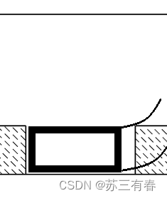
我们将地图纳入坐标轴中,以边界左侧顶点,即车位左侧最外点作为坐标原点(0,0),根据题目给出的车位宽2.4米,长5.1米,各边界的函数,一共有6条边界,图中圆圈为原点:
给出上述图形的代码:
这段代码是用来记录边界信息,即碰撞边界:
%% 边界信息
function wall=getbound()
global pos_Len pos_Wid road_Wid;
wall.bound{1}.line=[-pos_Len,0; 0,0];
wall.bound{2}.line=[0,0; 0,-pos_Wid];
wall.bound{3}.line=[0, pos_Len; -pos_Wid,-pos_Wid];
wall.bound{4}.line=[pos_Len, pos_Len; -pos_Wid,0];
wall.bound{5}.line=[pos_Len, 2*pos_Len; 0,0];
wall.bound{6}.line=[-pos_Len, 2*pos_Len; road_Wid,road_Wid];
wall.num=6;
end
这段代码是用来画车位的:
% 画车位
figure(1); hold on; box on; axis equal;
plotbox([-pos_Len,-pos_Wid,pos_Len,pos_Wid])
plotbox([pos_Len,-pos_Wid,pos_Len,pos_Wid])
% rectangle('Position',[-pos_Len,-pos_Wid,pos_Len,pos_Wid],'Linewidth',2,'LineStyle','-','EdgeColor','k');
% rectangle('Position',[pos_Len,-pos_Wid,pos_Len,pos_Wid],'Linewidth',1,'LineStyle','-','EdgeColor','k');
plot([0,pos_Len],[-pos_Wid,-pos_Wid],'k-','Linewidth',1);
plot([-pos_Len,2*pos_Len],[road_Wid,road_Wid],'k-','Linewidth',1);
wall=getbound();
这段代码用来画盒子:
%% 画盒子
function h=plotbox(box)
xdata = [box(1); box(1)+box(3); box(1)+box(3); box(1)];
ydata = [box(2); box(2); box(2)+box(4); box(2)+box(4)];
[h,g] = crosshatch_poly(xdata, ydata, 45, 0.25, 'hold', 1, ...'edgestyle', '-', 'edgecolor', 'k', 'edgewidth', 1, ...'linestyle', '--', 'linecolor', 'k', 'linewidth', 0.5);
end
建立车辆模型
我们需要将车辆的所有信息都表示在车辆模型中,包括:车长,车宽,车轴长,车轴宽,我们在车辆前轮加入车轮方向,在车辆后轮加入一个车身方向以及车身方向的法向量,以便后续计算。
给出车辆模型的代码:
这段代码用于计算车辆信息,包括车轮方向向量,车身方向向量,车身方向的法向量,车后轮位置,车前轮位置等等
%% 计算车辆信息
function car=carinfo(car)
% 已知车辆后轴中心和前进单位向量 car.back_cen car.body_e
% 求车辆四个顶点的信息
global car_Cen_Head car_Wid car_Cen_Cen;
car.head_cen=car.back_cen+car_Cen_Cen*car.body_e;
car.body_w=[cos(pi/2), -sin(pi/2); sin(pi/2), cos(pi/2)]*car.body_e; % 车辆的左侧方向
car.weel_e=[cos(car.weel_alpha), -sin(car.weel_alpha); sin(car.weel_alpha), cos(car.weel_alpha)]*car.body_e; % 车辆的车轮方向
car.v1=-car_Cen_Head*car.body_e-car_Wid*car.body_w/2;
car.v2=-car_Cen_Head*car.body_e+car_Wid*car.body_w/2;
car.v3= car_Cen_Head*car.body_e+car_Wid*car.body_w/2;
car.v4= car_Cen_Head*car.body_e-car_Wid*car.body_w/2;
car.box=[car.back_cen+car.v1, car.back_cen+car.v2, car.head_cen+car.v3, car.head_cen+car.v4];
car=getcarbound(car);
end
这段代码用于计算车辆边界,即车的长方形的框框
%% 计算车辆边界
function car=getcarbound(car)
car.bound{1}.line=[car.box(:,1:2)];
car.bound{2}.line=[car.box(:,2:3)];
car.bound{3}.line=[car.box(:,3:4)];
car.bound{4}.line=[car.box(:,[4,1])];
end
这段代码用于画汽车:
%% 画汽车
function h=plotcar(car)
h{1}=plot(car.back_cen(1),car.back_cen(2),'ro');
h{2}=plot(car.head_cen(1),car.head_cen(2),'r>');
h{3}=patch(car.box(1,:),car.box(2,:),'-','EdgeColor','k','FaceColor','non');
h{4}=plot([car.back_cen(1),car.back_cen(1)+car.body_e(1)],[car.back_cen(2),car.back_cen(2)+car.body_e(2)],'k-');
h{5}=plot([car.back_cen(1),car.back_cen(1)+car.body_w(1)],[car.back_cen(2),car.back_cen(2)+car.body_w(2)],'m-');
h{6}=plot([car.head_cen(1),car.head_cen(1)+car.weel_e(1)],[car.head_cen(2),car.head_cen(2)+car.weel_e(2)],'b-');
end
这段代码用于清除汽车,因为我们画图用getframe()函数,是将多个图片堆叠在一起的,如果不清楚每一次的车辆,则会将每一张图片的汽车都画上去。(若想看汽车的运动轨迹,车身运动时所占用的范围,就不需要清除汽车)
%% 清除汽车
function clearcar(h)
for i=1:length(h)delete(h{i});
end
end
现在我们将地图和车辆都画好了,下面我们写碰撞检测以及遍历的代码
碰撞检测以及遍历
下面的代码为碰撞检测,即判断车辆的边界与碰撞边界是否发生重合,在坐标系中,边界的碰撞可以比较两直线函数的大小即可
%% 碰撞检测
function [flag,car]=test(car,wal)
car=move_step(car);
car=carinfo(car);
car=getcarbound(car);
flag=0;
for i=1:4f=@(x,y) (y-car.bound{i}.line(2,1))*(car.bound{i}.line(1,2)-car.bound{i}.line(1,1))-...(x-car.bound{i}.line(1,1))*(car.bound{i}.line(2,2)-car.bound{i}.line(2,1));for j=1:wal.numg=@(x,y) (y-wal.bound{j}.line(2,1))*(wal.bound{j}.line(1,2)-wal.bound{j}.line(1,1))-...(x-wal.bound{j}.line(1,1))*(wal.bound{j}.line(2,2)-wal.bound{j}.line(2,1));if f(wal.bound{j}.line(1,1),wal.bound{j}.line(2,1))*f(wal.bound{j}.line(1,2),wal.bound{j}.line(2,2))<0 && ...g(car.bound{i}.line(1,1),car.bound{i}.line(2,1))*g(car.bound{i}.line(1,2),car.bound{i}.line(2,2))<0flag=1; return;endend
end
end下面的代码为遍历代码,我们设定的是每次移动0.02米,每次移动按照规定的车轮方向以及车身方向行进的,这一段代码涉及到车轮与车身方向不一致时的运动,因车辆为阿克曼车型,仅前轮可以转动,则前轮转动时,后轮可能还在做直线运动,因此这里需要比较扎实的数学功底。
%% 移动一步(0.1米)
function car=move_step(car)
global car_Len car_alpha; step=0.02;
if car.back==1car.weel_e=[cos(car.weel_alpha), -sin(car.weel_alpha); sin(car.weel_alpha), cos(car.weel_alpha)]*car.body_e; % 轮子单位向量car.back_cen=car.back_cen+step*car.body_e;                                                                       % 移动step米后的后轴中心car.head_cen=car.head_cen+(-2*(car_Len-step)*cos(car.weel_alpha)+sqrt(4*(car_Len-step)^2*cos(car.weel_alpha)^2-4*((car_Len-step)^2-car_Len^2)))*car.weel_e/2; % 移动step米后的前轴中心car.body_e=[car.head_cen(1)-car.back_cen(1); car.head_cen(2)-car.back_cen(2)]; car.body_e=car.body_e/norm(car.body_e);                   % 车身的单位向量
elseif car.back==-1% plot(car.head_cen(1),car.head_cen(2),'k.');car.weel_e=[cos(car.weel_alpha), -sin(car.weel_alpha); sin(car.weel_alpha), cos(car.weel_alpha)]*car.body_e; % 轮子单位向量car.back_cen=car.back_cen-step*car.body_e;                                                                       % 移动step米后的后轴中心car.head_cen=car.head_cen-(2*(car_Len+step)*cos(car.weel_alpha)-sqrt(4*(car_Len+step)^2*cos(car.weel_alpha)^2-4*((car_Len+step)^2-car_Len^2)))*car.weel_e/2; % 移动step米后的前轴中心% plot(car.head_cen(1),car.head_cen(2),'k.');car.body_e=[car.head_cen(1)-car.back_cen(1); car.head_cen(2)-car.back_cen(2)]; car.body_e=car.body_e/norm(car.body_e);                   % 车身的单位向量
elseerror('move_step error!');
end
end
车辆初始状态
下面给出车辆初始状态的代码:
%% 车辆初始状态
car.back_cen=[car_Cen_Head+Dcar2wall; -pos_Wid/2];
car.body_e=[1;0]; % 车身单位向量
car.back=1; % 车辆前进、后退标志(前进为1,后退为-1)
car.weel_alpha=car_alpha; % 车辆的轮子角度
car=carinfo(car); h=plotcar(car);
% 行驶出车库的距离可以根据L的变化而增长
L=480;
dots=zeros(1,2);
i1=0;i2=0;i3=0;for i=1:L[flag,trycar]=test(car,wall);if flag==0car=trycar; clearcar(h); car=carinfo(car);h=plotcar(car);t=@(x)((car.box(2,4)-car.box(2,1))/(car.box(1,4)-car.box(1,1))*(x-car.box(1,1))+car.box(2,1));if(t(pos_Len)>0)
%                 break;
i3=i3+1;
car.weel_e=car.body_e;car.weel_alpha=0;clearcar(h); h=plotcar(car);car.back=1;fstraight=@(x)((x-car.back_cen(1))/(car.head_cen(1)-car.back_cen(1))*...(car.head_cen(2)-car.back_cen(2))+car.head_cen(2));y1=@(x)(-(car.box(1)-car.box(7))/(car.box(2)-car.box(8)))*(x-car.back_cen(1))+car.back_cen(2);end% d1=sqrt((car.back_cen(1)-5.4)^2+car.back_cen(2)^2)
%     y1(5.4);
%     if(y1(5.4)>0)
%         break;
%     endF(i)=getframe;% disp('forward');% disp(car.weel_alpha/pi*180);%         plot(car.head_cen,'.');%         plot(car.back_cen,'.');elsecar.back=-1*car.back; car.weel_alpha=-1*car.weel_alpha;car=carinfo(car);i1=i1+1;%         plot(car.head_cen,'-');%         plot(car.back_cen,'-');% disp('backward');% disp(car.weel_alpha/pi*180);
%             dot1=[dots1;car.back_cen(1),car.back_cen(2)];
% dots1=[dots1;dot1];enddot=[car.back_cen(1),car.back_cen(2)];dots=[dots;dot];endcar.weel_alpha=-470/16/180*pi; for i=1:200i2=i2+1;[flag,trycar]=test(car,wall);if flag==0car=trycar; clearcar(h); car=carinfo(car);h=plotcar(car);F(i)=getframe;if(car.body_e(2)<=0)break;endelsecar.back=-1*car.back; car.weel_alpha=-1*car.weel_alpha;car=carinfo(car);enddot=[car.back_cen(1),car.back_cen(2)];dots=[dots;dot];endfigure (2)plot(dots(2:end,1),dots(2:end,2),'b-');hold onx0=[dots(end,1),dots(end,2)]a=car.back_cen(2)-2.75此处除了初始状态外,还有整合调用其它代码的部分,也就是说,这段代码其实是整个代码的主体部分。
当然,代码中还有许多当初比赛时测试留下来的许多无用的注释和无用变量,笔者目前太累了已经没有精力去检查与改动,但这并不影响代码的运行。有兴趣的同学可以自行删除和修改,若能力有限的同学直接运行也是可以的。
至此,我们基本上完成了平行泊车的迭代测试碰撞代码,以不断前进后退改变方向的形式完成入库。完整代码我贴在最后面,先来看一下GIF动图:

最后的弹出的新图像为:

我们以后轮轴中心点作为控制点,该图像表明了在坐标系中,控制点的轨迹图像,在最开始部分,车辆不断地小规模挪动,等挪动到可以出去后,便直线运动离开车库。
下面附上完整代码:
完整代码
在给出完整代码之前:先要注意的是,建议在2018及以上版本的matlab中运行代码,因为各function全部放在一个脚本文件中,低版本matlab是不允许这样的,如果在低版本中运行的话,可以把function文件加入搜索路径。若还不行,则建议下载2018及以上版本。
MATLAB 2018b 安装与简介
上面链接的安装大致与我的安装相似(我是由学校学习通提供的安装包以及安装流程)
Prog.m代码:
clear,clc, close all;
addpath lib; R=4.97;
global car_Len car_Wid car_Weel_Den car_Cen_Cen; % 车辆参数
global car_alpha car_oil_ddt car_speed_dt car_speed_ddt car_FXP_speed bump_den bump_speed park_forward_Speed park_backward_Speed;
global pos_Len pos_Wid pos_Head road_Wid car_Cen_Head; % 车位和道路参数
car_Len=4.9; % 车长
car_Wid=1.8; % 车宽
car_Weel_Den=1.7; % 轮宽
car_Cen_Cen=2.8; % 轴距
car_alpha=470/16/180*pi; % 最大转角
car_oil_ddt=3; % 油门加速度
car_speed_dt=-6; % 最大刹车减速度
car_speed_ddt=20; % 最大加加速度
car_FXP_speed=400/180*pi; % 方向盘转动角速度
bump_den=5; % 减速带距离
bump_speed=10; % 减速带速度
park_forward_Speed=20;  % 汽车最大前进车速
park_backward_Speed=10;  % 汽车最大倒车车速
pos_Len=5.4; % 车位长度
pos_Wid=2.4; % 车位宽度
pos_Head=0.2; % 车位头部
road_Wid=5.5; % 道路宽度
car_Cen_Head=(car_Len-car_Cen_Cen)/2; % 车辆控制中心至车尾距离
Dcar2wall=0.00; % 车尾与墙的间距% 画车位
figure(1); hold on; box on; axis equal;
plotbox([-pos_Len,-pos_Wid,pos_Len,pos_Wid])
plotbox([pos_Len,-pos_Wid,pos_Len,pos_Wid])
% rectangle('Position',[-pos_Len,-pos_Wid,pos_Len,pos_Wid],'Linewidth',2,'LineStyle','-','EdgeColor','k');
% rectangle('Position',[pos_Len,-pos_Wid,pos_Len,pos_Wid],'Linewidth',1,'LineStyle','-','EdgeColor','k');
plot([0,pos_Len],[-pos_Wid,-pos_Wid],'k-','Linewidth',1);
plot([-pos_Len,2*pos_Len],[road_Wid,road_Wid],'k-','Linewidth',1);
wall=getbound();%% 车辆初始状态
car.back_cen=[car_Cen_Head+Dcar2wall; -pos_Wid/2];
car.body_e=[1;0]; % 车身单位向量
car.back=1; % 车辆前进、后退标志(前进为1,后退为-1)
car.weel_alpha=car_alpha; % 车辆的轮子角度
car=carinfo(car); h=plotcar(car);
% 行驶出车库的距离可以根据L的变化而增长
L=480;
dots=zeros(1,2);
i1=0;i2=0;i3=0;for i=1:L[flag,trycar]=test(car,wall);if flag==0car=trycar; clearcar(h); car=carinfo(car);h=plotcar(car);t=@(x)((car.box(2,4)-car.box(2,1))/(car.box(1,4)-car.box(1,1))*(x-car.box(1,1))+car.box(2,1));if(t(pos_Len)>0)
%                 break;
i3=i3+1;
car.weel_e=car.body_e;car.weel_alpha=0;clearcar(h); h=plotcar(car);car.back=1;fstraight=@(x)((x-car.back_cen(1))/(car.head_cen(1)-car.back_cen(1))*...(car.head_cen(2)-car.back_cen(2))+car.head_cen(2));y1=@(x)(-(car.box(1)-car.box(7))/(car.box(2)-car.box(8)))*(x-car.back_cen(1))+car.back_cen(2);end% d1=sqrt((car.back_cen(1)-5.4)^2+car.back_cen(2)^2)
%     y1(5.4);
%     if(y1(5.4)>0)
%         break;
%     endF(i)=getframe;% disp('forward');% disp(car.weel_alpha/pi*180);%         plot(car.head_cen,'.');%         plot(car.back_cen,'.');elsecar.back=-1*car.back; car.weel_alpha=-1*car.weel_alpha;car=carinfo(car);i1=i1+1;%         plot(car.head_cen,'-');%         plot(car.back_cen,'-');% disp('backward');% disp(car.weel_alpha/pi*180);
%             dot1=[dots1;car.back_cen(1),car.back_cen(2)];
%             dots1=[dots1;dot1];enddot=[car.back_cen(1),car.back_cen(2)];dots=[dots;dot];endcar.weel_alpha=-470/16/180*pi;   for i=1:200i2=i2+1;[flag,trycar]=test(car,wall);if flag==0car=trycar; clearcar(h); car=carinfo(car);h=plotcar(car);F(i)=getframe;if(car.body_e(2)<=0)break;endelsecar.back=-1*car.back; car.weel_alpha=-1*car.weel_alpha;car=carinfo(car);enddot=[car.back_cen(1),car.back_cen(2)];dots=[dots;dot];endfigure (2)plot(dots(2:end,1),dots(2:end,2),'b-');hold onx0=[dots(end,1),dots(end,2)]a=car.back_cen(2)-2.75
%% 碰撞检测
function [flag,car]=test(car,wal)
car=move_step(car);
car=carinfo(car);
car=getcarbound(car);
flag=0;
for i=1:4f=@(x,y) (y-car.bound{i}.line(2,1))*(car.bound{i}.line(1,2)-car.bound{i}.line(1,1))-...(x-car.bound{i}.line(1,1))*(car.bound{i}.line(2,2)-car.bound{i}.line(2,1));for j=1:wal.numg=@(x,y) (y-wal.bound{j}.line(2,1))*(wal.bound{j}.line(1,2)-wal.bound{j}.line(1,1))-...(x-wal.bound{j}.line(1,1))*(wal.bound{j}.line(2,2)-wal.bound{j}.line(2,1));if f(wal.bound{j}.line(1,1),wal.bound{j}.line(2,1))*f(wal.bound{j}.line(1,2),wal.bound{j}.line(2,2))<0 && ...g(car.bound{i}.line(1,1),car.bound{i}.line(2,1))*g(car.bound{i}.line(1,2),car.bound{i}.line(2,2))<0flag=1; return;endend
end
end%% 移动一步(0.02米)
function car=move_step(car)
global car_Len car_alpha; step=0.02;
if car.back==1car.weel_e=[cos(car.weel_alpha), -sin(car.weel_alpha); sin(car.weel_alpha), cos(car.weel_alpha)]*car.body_e; % 轮子单位向量car.back_cen=car.back_cen+step*car.body_e;                                                                       % 移动step米后的后轴中心car.head_cen=car.head_cen+(-2*(car_Len-step)*cos(car.weel_alpha)+sqrt(4*(car_Len-step)^2*cos(car.weel_alpha)^2-4*((car_Len-step)^2-car_Len^2)))*car.weel_e/2; % 移动step米后的前轴中心car.body_e=[car.head_cen(1)-car.back_cen(1); car.head_cen(2)-car.back_cen(2)]; car.body_e=car.body_e/norm(car.body_e);                   % 车身的单位向量
elseif car.back==-1% plot(car.head_cen(1),car.head_cen(2),'k.');car.weel_e=[cos(car.weel_alpha), -sin(car.weel_alpha); sin(car.weel_alpha), cos(car.weel_alpha)]*car.body_e; % 轮子单位向量car.back_cen=car.back_cen-step*car.body_e;                                                                       % 移动step米后的后轴中心car.head_cen=car.head_cen-(2*(car_Len+step)*cos(car.weel_alpha)-sqrt(4*(car_Len+step)^2*cos(car.weel_alpha)^2-4*((car_Len+step)^2-car_Len^2)))*car.weel_e/2; % 移动step米后的前轴中心% plot(car.head_cen(1),car.head_cen(2),'k.');car.body_e=[car.head_cen(1)-car.back_cen(1); car.head_cen(2)-car.back_cen(2)]; car.body_e=car.body_e/norm(car.body_e);                   % 车身的单位向量
elseerror('move_step error!');
end
end% plot([car.back_cen(1),car.back_cen(1)+car.e(1)],[car.back_cen(2),car.back_cen(2)+car.e(2)],'r-');
% plot([car.back_cen(1),car.back_cen(1)+car.w(1)],[car.back_cen(2),car.back_cen(2)+car.w(2)],'b-');%% 计算车辆信息
function car=carinfo(car)
% 已知车辆后轴中心和前进单位向量 car.back_cen car.body_e
% 求车辆四个顶点的信息
global car_Cen_Head car_Wid car_Cen_Cen;
car.head_cen=car.back_cen+car_Cen_Cen*car.body_e;
car.body_w=[cos(pi/2), -sin(pi/2); sin(pi/2), cos(pi/2)]*car.body_e; % 车辆的左侧方向
car.weel_e=[cos(car.weel_alpha), -sin(car.weel_alpha); sin(car.weel_alpha), cos(car.weel_alpha)]*car.body_e; % 车辆的车轮方向
car.v1=-car_Cen_Head*car.body_e-car_Wid*car.body_w/2;
car.v2=-car_Cen_Head*car.body_e+car_Wid*car.body_w/2;
car.v3= car_Cen_Head*car.body_e+car_Wid*car.body_w/2;
car.v4= car_Cen_Head*car.body_e-car_Wid*car.body_w/2;
car.box=[car.back_cen+car.v1, car.back_cen+car.v2, car.head_cen+car.v3, car.head_cen+car.v4];
car=getcarbound(car);
end%% 计算车辆边界
function car=getcarbound(car)
car.bound{1}.line=[car.box(:,1:2)];
car.bound{2}.line=[car.box(:,2:3)];
car.bound{3}.line=[car.box(:,3:4)];
car.bound{4}.line=[car.box(:,[4,1])];
end%% 边界信息
function wall=getbound()
global pos_Len pos_Wid road_Wid;
wall.bound{1}.line=[-pos_Len,0; 0,0];
wall.bound{2}.line=[0,0; 0,-pos_Wid];
wall.bound{3}.line=[0, pos_Len; -pos_Wid,-pos_Wid];
wall.bound{4}.line=[pos_Len, pos_Len; -pos_Wid,0];
wall.bound{5}.line=[pos_Len, 2*pos_Len; 0,0];
wall.bound{6}.line=[-pos_Len, 2*pos_Len; road_Wid,road_Wid];
wall.num=6;
end%% 画汽车
function h=plotcar(car)
h{1}=plot(car.back_cen(1),car.back_cen(2),'ro');
h{2}=plot(car.head_cen(1),car.head_cen(2),'r>');
h{3}=patch(car.box(1,:),car.box(2,:),'-','EdgeColor','k','FaceColor','non');
h{4}=plot([car.back_cen(1),car.back_cen(1)+car.body_e(1)],[car.back_cen(2),car.back_cen(2)+car.body_e(2)],'k-');
h{5}=plot([car.back_cen(1),car.back_cen(1)+car.body_w(1)],[car.back_cen(2),car.back_cen(2)+car.body_w(2)],'m-');
h{6}=plot([car.head_cen(1),car.head_cen(1)+car.weel_e(1)],[car.head_cen(2),car.head_cen(2)+car.weel_e(2)],'b-');
end%% 清除汽车
function clearcar(h)
for i=1:length(h)delete(h{i});
end
end%% 画盒子
function h=plotbox(box)
xdata = [box(1); box(1)+box(3); box(1)+box(3); box(1)];
ydata = [box(2); box(2); box(2)+box(4); box(2)+box(4)];
[h,g] = crosshatch_poly(xdata, ydata, 45, 0.25, 'hold', 1, ...'edgestyle', '-', 'edgecolor', 'k', 'edgewidth', 1, ...'linestyle', '--', 'linecolor', 'k', 'linewidth', 0.5);
end
crosshatch_poly.m代码,这段代码是在画盒子时需要调用的额外的函数:
function [h,g] = crosshatch_poly(x, y, lineangle, linegap, varargin)
% Fill a convex polygon with regular diagonal lines (hatching, or cross-hatching)
%
% file:      	crosshatch_poly.m, (c) Matthew Roughan, Mon Jul 20 2009
% created: 	Mon Jul 20 2009
% author:  	Matthew Roughan
% email:   	matthew.roughan@adelaide.edu.au
%
%
% crosshatch_poly(x, y, angle, gap) fills the 2-D polygon defined by vectors x and y
% with slanted lines at the specified lineangle and linegap.
%
% The one major limitation at present is that the polygon must be convex -- if it is not, the
% function will fill the convex hull of the supplied vertices. Non-convex polygons must be
% broken into convex chunks, which is a big limitation at present.
%
% Cross-hatching can be easily achieved by calling the function twice.
%
% Speckling can be roughly achieved using linestyle ':'
%
%
% INPUTS:
%     (x,y)  gives a series of points that defines a convex polygon.
%     lineangle  the angle of the lines used to fill the polygon
%            specified in degrees with respect to vertical
%            default = 45 degrees
%     linegap    the gap between the lines used to fill the polygon
%            default = 1
%     options can be specified in standard Matlab (name, value) pairs
%        'edgecolor'  color of the boundary line of the polygon
%        'edgewidth'  width of the boundary line of the polygon
%                         0 means no line
%        'edgestyle'  style of the boundary line of the polygon
%        'linecolor'  color of the fill lines
%        'linewidth'  width of fill lines
%        'linestyle'  style of fill lines
%        'backgroundcolor'  background colour to fill the polygon with
%                     if not specified, no fill will be done
%        'hold_n'     hold_n=1 means keep previous plot
%                     hold_n=0 (default) means clear previous figure
%
% OUTPUTS:
%    h = a vector of handles to the edges of the polygon
%    g = a vector of handles to the lines
%
% Works by finding intersection points of the fill lines with the boundary lines, and then
% drawing a line between intersection points that lie on the boundary of the polygon.
%
% version 0.1, Jul 20th 2009, Matthew Roughan
% version 0.2, Jul 22nd 2009, fixed typo, Matthew Roughan
%
%
% There are a number of similar functions, that I'll point to, but they are a little
% different as well.
%    linpat.m by Stefan Bilig does essentially the same thing, but only in rectangular regions
%    applyhatch_pluscolor.m by Brandon Levey (from Brian Katz and Ben Hilig) maps colors in
%             an image to patterns, which is cool, but I just want hatching to be easy, and
%             direct, so I can do things like plot two regions and cross hatch both
%    hatching.m by  ijtihadi ijtihadi does hatching between two (arbitrary) functions, which
%             could include many shapes, but isn't easy to use directly for polygons or other
%             shapes. Note that often smooth curves can be well approximated by polygons so
%             this function can be used for these cases as well.
%
%
% TODO: speckles and other more interesting patterns
%       cross-hatching as a built in
%       avoid dependence on optimization toolbox
% % read the input options and set defaults
if (nargin < 4)linegap = 1;
end
if (nargin < 3)lineangle = 45;
end
edgecolor = 'k';
edgewidth = 1;
edgestyle = '-';
linecolor = 'k';
linewidth = 1;
linestyle = '-';
hold_n = 0;
if (length(varargin) > 0)% process variable argumentsfor k = 1:2:length(varargin)if (ischar(varargin{k}))argument = char(varargin{k}); value = varargin{k+1};switch argumentcase {'linecolor','lc'}linecolor = value;case {'backgroundcolor','bgc'}backgroundcolor = value;case {'linewidth','lw'}linewidth = value;case {'linestyle','ls'}linestyle = value;case {'edgecolor','ec'}edgecolor = value;case {'edgewidth','ew'}edgewidth = value;case {'edgestyle','ew'}edgestyle = value;case {'hold'}hold_n = value;otherwiseerror('incorrect input parameters');endendend
end% reset plot of needed
if (hold_n==0)hold offplot(x(1), y(2));
end
hold on% get the convex hull of the supplied vertices, partly to ensure convexity, but also to sort
% them into a sensible order
[k] = convhull(x,y);
x = x(k(1:end-1));
y = y(k(1:end-1));
N = length(k)-1;
% make everything row vectors
if (size(x,1) > 1)x = x';
end
if (size(y,1) > 1)y = y';
end% if the background is set, then fill, and set the edge correctly
if (exist('backgroundcolor', 'var'))h = fill(x,y,backgroundcolor);if (edgewidth > 0)set(h, 'LineWidth', edgewidth, 'EdgeColor', edgecolor, 'LineStyle', edgestyle);elseset(h, 'EdgeColor', backgroundcolor);end
end% plot edges if needed
for i=1:Nif (edgewidth > 0 & ~exist('backgroundcolor', 'var'))% only need to draw edges if width is > 0 and haven't already done so with fillj = mod(i, N)+1;h(i) = plot([x(i) x(j)], [y(i) y(j)], ...'color', edgecolor, 'linestyle', edgestyle, 'linewidth', edgewidth);end
end% now find the range for the lines to plot
c = [cosd(lineangle), sind(lineangle)];  % normal to the lines
v = [sind(lineangle), -cosd(lineangle)]; % direction of lines
obj = c * [x; y];
[mx, kmx] = max(obj, [], 2);
[mn, kmn] = min(obj, [], 2);
% plot(x(kmx), y(kmx), 'r*');
% plot(x(kmn), y(kmn), 'ro');
distance = sqrt( (x(kmx)-x(kmn)).^2 + (y(kmx)-y(kmn)).^2  );% find a line describing each edge
for i=1:Nj = mod(i, N)+1;if (abs(x(j) - x(i)) > 1.0e-12)% find the slope and interseptslope(i) = (y(j) - y(i)) / (x(j) - x(i));y_int(i) = y(i) - slope(i)*x(i);else% the line is verticalslope(i) = Inf;y_int(i) = NaN;end
end% now draw lines clipping them at points that are on the edge of the polygon
g = [];
% find a slightly larger polygon
centroid_x = mean(x);
centroid_y = mean(y);
epsilon = 0.001;
x_dash = (1+epsilon) * (x - centroid_x) + centroid_x;
y_dash = (1+epsilon) * (y - centroid_y) + centroid_y;
% fill(x_dash, y_dash, 'g');
for m=0:linegap:distancecounter = ceil(m/linegap)+1;sigma = [x(kmn), y(kmn)] + m*c;% plot(sigma(1), sigma(2), '+', 'color', linecolor);% for each line, look where it intersepts the edge of polygon (if it does)for i=1:N% find the intercept with this line, and the relevant edgeif (isinf(slope(i)))if (abs(v(1)) > 1.0e-12)t = (x(i) - sigma(1)) / v(1);x_i(i) = x(i);y_i(i) = sigma(2) + t * v(2);elsex_i(i) = NaN;y_i(i) = NaN;endelseif (abs(v(2) - slope(i)*v(1)) > 1.0e-12)t = (slope(i) * sigma(1) - sigma(2) + y_int(i)) / ( v(2) - slope(i)*v(1));x_i(i) = sigma(1) + t * v(1);y_i(i) = sigma(2) + t * v(2);elsex_i(i) = NaN;y_i(i) = NaN;endendendk = find(inpolygon(x_i, y_i, x_dash, y_dash));if (length(k) == 2)g(counter) = plot(x_i(k), y_i(k), ...'color', linecolor, 'linestyle', linestyle, 'linewidth', linewidth);elseif (length(k) < 2)% don't plot because we have no clear lineelseif (length(k) > 2)% find two unique pointsd = [x_i(k)', y_i(k)'];d = round(100*d)/100;d = unique(d, 'rows');g(counter) = plot(d(:,1), d(:,2), ...'color', linecolor, 'linestyle', linestyle, 'linewidth', linewidth);hold on;end
end若你的matlab版本在2018及以上,则将两段代码分别复制创建成两个m文件,运行第一个代码即可。
如果你看到这里,真的非常感谢!希望我的博客能给你提供一点小小的帮助!