逻辑回归算法实现

article/2025/9/16 17:53:56

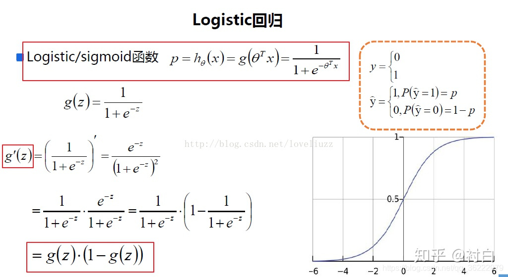
逻辑回归算法原理还是比较容易理解的，根据计算的结果实现一下：

手写的推导过程如下：

然后我们开始写实现的过程

1、写出判断模型准确性的函数，这个比较容易理解

import numpy as np
from math import sqrtdef accuracy_score(y_true, y_predict):"""计算y_true和y_predict之间的准确率"""assert len(y_true) == len(y_predict), \"the size of y_true must be equal to the size of y_predict"return np.sum(y_true == y_predict) / len(y_true)

2、写出来训练数据集和测试数据集的分割函数，这个也可以直接用sklearn中写好的包

import numpy as npdef train_test_split(X, y, test_ratio=0.2, seed=None):"""将数据 X 和 y 按照test_ratio分割成X_train, X_test, y_train, y_test"""assert X.shape[0] == y.shape[0], \"the size of X must be equal to the size of y"assert 0.0 <= test_ratio <= 1.0, \"test_ration must be valid"if seed:np.random.seed(seed)shuffled_indexes = np.random.permutation(len(X))test_size = int(len(X) * test_ratio)test_indexes = shuffled_indexes[:test_size]train_indexes = shuffled_indexes[test_size:]X_train = X[train_indexes]y_train = y[train_indexes]X_test = X[test_indexes]y_test = y[test_indexes]return X_train, X_test, y_train, y_test

3、写出函数的fit过程，求解用的是批量梯度下降法，这个过程和线性回归比较类似

import numpy as npclass LogisticRegression:def __init__(self):"""初始化模型"""self.coef_ = Noneself.intercept_ = Noneself._theta = None#有下划线是私有函数def _sigmod(self,t):return 1./(1.+np.exp(-t))def fit(self,X_train,y_train,eta=0.01,n_iters=1e4):"""根据模型训练数据集X_train,y_train,使用梯度下降法训练Logistic Regression"""assert X_train.shape[0] == y_train.shape[0],\"the size of X_train must be equal to the size of y_trian"#计算损失函数def J(theta,X_b,y):y_hat = self._sigmod(X_b.dot(theta))try:return -np.sum(y*np.log(y_hat) + (1-y)*np.log(1-y_hat))/ len(y)except:return float("inf")def dJ(theta,X_b,y):return X_b.T.dot(self._sigmod(X_b.dot(theta))-y) / len(X_b)def gradient_descent(X_b, y, inital_theta, eta, n_inters=1e4, epsilon=1e-8):theta = initial_thetai_inter = 0while i_inter < n_inters:gradient = dJ(theta, X_b, y)last_theta = thetatheta = theta - eta * gradientif (abs(J(theta, X_b, y) - J(last_theta, X_b, y)) < epsilon):breaki_inter += 1return thetaX_b = np.hstack([np.ones((len(X_train),1)),X_train])initial_theta = np.zeros(X_b.shape[1])self._theta = gradient_descent(X_b,y_train,initial_theta,eta,n_iters)self.intercept_ = self._theta[0]self.coef_ = self._theta[1:]return self

4、写出来预测的概率和预测的分类结果

    #预测的概率函数def predict_proba(self,X_predict):"""给定待预测数据集X_predict,返回X_predict的结果向量"""assert self.intercept_ is not None and self.coef_ is not None,\"Must fit before predixt"assert X_predict.shape[1] == len(self.coef_),\"the feature number of X_predict must be equal to X_train"X_b = np.hstack([np.ones((len(X_predict),1)), X_predict])return  self._sigmod(X_b.dot(self._theta))#预测结果的函数def predict(self,X_predict):"""给定预测数据集X_predict,返回表示X_predict的结果向量"""assert self.intercept_ is not None and self.coef_ is not None,\"Must fit before predixt"assert X_predict.shape[1] == len(self.coef_),\"the feature number of X_predict must be equal to X_train"proba = self.predict_proba(X_predict)return np.array(proba >= 0.5, dtype='int')def score(self, X_test, y_test):"""根据测试数据集X_test和y_test确定当前模型的准确度"""y_predict = self.predict(X_test)return accuracy_score(y_test,y_predict)def __repr__(self):return  "LogisticRegression()"

5、然后用iris数据集验证下我们写的函数

import numpy as np
import matplotlib.pyplot as plt
from sklearn import datasets
from sklearn.model_selection import train_test_splitiris = datasets.load_iris()
X = iris.data
y = iris.targetX = X[y<2, :2]
y = y[y<2]plt.scatter(X[y ==0,0],X[y==0,1],color='red')
plt.scatter(X[y ==1,0],X[y==1,1],color='blue')
plt.show()X_train,X_test,y_train,y_test = train_test_split(X,y)log_reg = LogisticRegression()
log_reg.fit(X_train,y_train)log_reg.score(X_test,y_test)

结果如下：