引言

逻辑回归（Logistic Regression）是一种分类学习算法，其本质是将样本的特征和样本发生的概率联系起来，由于发生的概率是一个数值，因此称为回归算法。主要解决2分类问题，例如：一个垃圾邮件过滤系统，x是邮件的特征，预测的y值就是邮件的类别（是垃圾邮件还是正常邮件）。

逻辑回归算法原理

逻辑回归算法步骤如下

1. 计算样本发生的概率值，即 $\hat{p}=f(x)$
2. 根据样本发生的概率分类$$\hat{y}=\{\begin{array}{l}1，\hat{p}\ge 0.5\\ 0，\hat{p}\le 0.5\end{array}$$

逻辑回归算法既可以看作回归算法，也可以看作分类算法，只执行第一步时就是回归算法，但是逻辑回归算法通常作为回归算法用，主要解决2分类问题。在线性回归算法中，样本预测值
$$\hat{y}=f(x)={\theta }^T\cdot x_b$$
其值域为($-\infty ,+\infty$)，而概率的值域为[0,1],因此需要对$f(x)$函数进行处理，使之值域处于[0,1]
即$\hat{p}=\sigma ({\theta }^T\cdot x_b)$，一般
$$\sigma (t)=\frac{1}{1+e^{-t}}$$

$\sigma (t)$值域为（0,1），当t>0时，p>0.5；当t<0时，p<0.5

逻辑回归损失函数

模型预测值 $\hat{y}$ 如下
$$\hat{y}=\{\begin{array}{l}1，\hat{p}\ge 0.5\\ 0，\hat{p}\le 0.5\end{array}$$
由此可以看出当实际值y=1时，p越小，损失越大；当y=0时，p越大，损失越大，即
$$cost=\{\begin{array}{l}y=1时，p越小，损失越大\\ y=0时，p越大，损失越大\end{array}$$

下面函数刚好满足条件

$$cost=\{\begin{array}{l}-log(\hat{p})，ify=1\\ -log(1-\hat{p})，ify=0\end{array}$$
画出cost函数图像可以看出，当样本实际值为1时，预测概率值x为0，$-\log (x)$趋于正无穷，即损失趋于正无穷，当x=1即符合实际值，损失为0；当样本实际值为0时，预测值概率值x为1，$-\log (1-x)$趋于正无穷，即损失趋于正无穷，当x=0即符合实际值，损失为0。

损失函数可以合为1个，即

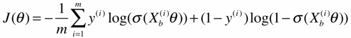
最终得到损失函数
$$J(\theta )=-\frac{1}{m}\sum _{i=1}^m{y}^{(i)}+\log ({\hat{p}}^{(i)})+(1-y^{(i)})\log (1-{\hat{p}}^{(i)})$$

$${\hat{p}}^{(i)}=\sigma (X_b^{(i)}\theta )=\frac{1}{1+e^{-X_b^{(i)}\theta }}$$

最后可以通过梯度下降法，求出使损失函数最小的$\theta$，求得的损失函数梯度如下

python实现逻辑回归

import numpy as np
import matplotlib.pyplot as plt
from sklearn.datasets import load_iris
from sklearn.model_selection import train_test_splitclass LogisticRegression:def __init__(self):self.coef_ = Noneself.intercept_ = Noneself._theta = Nonedef _sigmoid(self, t):return 1 / (1 + np.exp(-t))def fit(self, x_train, y_trian, n):def J(theta, x_b, y):y_hat = self._sigmoid(x_b.dot(theta))return -np.sum(y * np.log(y_hat) + (1 - y) * np.log(1 - y_hat)) / len(y)def dJ(theta, x_b, y):return x_b.T.dot(self._sigmoid(x_b.dot(theta)) - y) / len(y)def gradient_descent(x_b, y, initial_theta, alpha=0.01, n_iters=1e4, epsilon=1e-8):theta = initial_thetaiter = 0while iter < n_iters:gradient = dJ(theta, x_b, y)last_theta = thetatheta = theta - alpha * gradientif abs(J(last_theta, x_b, y) - J(theta, x_b, y)) < epsilon:breakiter += 1return last_thetax_b = np.hstack([np.ones((len(x_train), 1)), x_train])initail_theta = np.zeros(x_b.shape[1])self._theta = gradient_descent(x_b, y_trian, initail_theta, n_iters=n)self.intercept_ = self._theta[0]self.coef_ = self._theta[1:]def predict_prob(self, x_test):x_b = np.hstack([np.ones((len(x_test), 1)), x_test])return self._sigmoid(x_b.dot(self._theta))def predict(self, x_test):prob = self.predict_prob(x_test)return np.array(prob >= 0.5,dtype='int')def score(self, x_test, y_test):return np.sum(y_test == self.predict(x_test)) / len(y_test)# 鸢尾花数据集测试手写逻辑回归算法
iris = load_iris()
x = iris.data
y = iris.target# 由于逻辑回归只能处理2分类问题，截取分类为0,1，保留x2个特征方便可视化
X = x[y < 2, :2]
Y = y[y < 2]plt.scatter(X[Y == 0, 0], X[Y == 0, 1])
plt.scatter(X[Y == 1, 0], X[Y == 1, 1], color='r')
plt.show()x_train, x_test, y_train, y_test = train_test_split(X, Y)logistic = LogisticRegression()
logistic.fit(x_train, y_train, n=1e6)
y_predict = logistic.predict(x_test)
score = logistic.score(x_test, y_test)
print(score)
print(y_predict)
print(y_test)

输出
1.0
[0 1 1 1 0 0 0 0 0 1 1 0 1 1 1 0 0 1 1 0 1 0 1 1 1]
[0 1 1 1 0 0 0 0 0 1 1 0 1 1 1 0 0 1 1 0 1 0 1 1 1]

决策边界

决策边界就是能够把样本正确分类的一条边界
$$\hat{p}=\sigma (X_b\cdot \theta )=\frac{1}{1+e^{-X_b\cdot \theta }}$$
$$\hat{y}=\{\begin{array}{l}1，\hat{p}\ge 0.5\\ 0，\hat{p}\le 0.5\end{array}$$
当$\hat{p}=0.5$时，=>$X_b\cdot \theta =0$， 即为决策边界

(1) 当样本空间只有2个特征情况，即

$${\theta }_0+x_1{\theta }_1+x_2{\theta }_2=0$$

$$x_2=\frac{-{\theta }_0-x_1{\theta }_1}{{\theta }_2}$$
绘制$x_1,x_2$关系直线图

x_1 = np.linspace(4, 7, 100)
x_2 = (-logistic.intercept_ - x_1 * logistic.coef_[0]) / logistic.coef_[1]
plt.plot(x_1, x_2)
plt.show()

（2）不规则决策边界绘制
把整个区域看成无数个点，用得出的模型去预测这些点，不同分类用不同颜色区分

def plot_decision_boundary(model, axis):# x/y轴矩阵，如x:0-2,y:0-1,得到x=[[0, 1, 2],[0, 1, 2]],y=[[0, 0, 0],[1, 1, 1]]x, y = np.meshgrid(np.linspace(axis[0], axis[1], int((axis[1] - axis[0]) * 100)).reshape(-1, 1),np.linspace(axis[2], axis[3], int((axis[3] - axis[2]) * 100)).reshape(-1, 1))# 矩阵拼接，如x:0-2,y:0-1,得到[[0. 0.], [1. 0.], [2. 0.], [0. 1.], [1. 1.], [2. 1.]]x_new = np.c_[x.reshape(-1), y.reshape(-1)]y_predict = model.predict(x_new)zz = y_predict.reshape(x.shape)custom_cmap = ListedColormap(['#EF9A9A', '#EFF59D', '#90CAF9'])plt.contourf(x, y, zz, linewidth=5, cmap=custom_cmap)

python实现多项式逻辑回归

import numpy as np
import matplotlib.pyplot as plt
from sklearn.pipeline import Pipeline
from sklearn.model_selection import train_test_split
from sklearn.preprocessing import PolynomialFeatures
from sklearn.preprocessing import StandardScalerclass LogisticRegression:def __init__(self):self.coef_ = Noneself.intercept_ = Noneself._theta = Nonedef _sigmoid(self, t):return 1 / (1 + np.exp(-t))def fit(self, x_train, y_trian, n=1e4):def J(theta, x_b, y):y_hat = self._sigmoid(x_b.dot(theta))return -np.sum(y * np.log(y_hat) + (1. - y) * np.log(1. - y_hat)) / len(y)def dJ(theta, x_b, y):return x_b.T.dot(self._sigmoid(x_b.dot(theta)) - y) / len(x_b)def gradient_descent(x_b, y, initial_theta, alpha=0.01, n_iters=1e4, epsilon=1e-8):theta = initial_thetaiter = 0while iter < n_iters:gradient = dJ(theta, x_b, y)last_theta = thetatheta = theta - alpha * gradientif abs(J(last_theta, x_b, y) - J(theta, x_b, y)) < epsilon:breakiter += 1return last_thetax_b = np.hstack([np.ones((len(x_train), 1)), x_train])initail_theta = np.zeros(x_b.shape[1])self._theta = gradient_descent(x_b, y_trian, initail_theta, n_iters=n)self.intercept_ = self._theta[0]self.coef_ = self._theta[1:]def predict_prob(self, x_test):x_b = np.hstack([np.ones((len(x_test), 1)), x_test])return self._sigmoid(x_b.dot(self._theta))def predict(self, x_test):prob = self.predict_prob(x_test)return np.array(prob >= 0.5, dtype='int')def score(self, x_test, y_test):return np.sum(y_test == self.predict(x_test)) / len(y_test)def plot_decision_boundary(model, axis):# x/y轴矩阵，如x:0-2,y:0-1,得到x=[[0, 1, 2],[0, 1, 2]],y=[[0, 0, 0],[1, 1, 1]]x, y = np.meshgrid(np.linspace(axis[0], axis[1], int((axis[1] - axis[0]) * 100)).reshape(-1, 1),np.linspace(axis[2], axis[3], int((axis[3] - axis[2]) * 100)).reshape(-1, 1))# 矩阵拼接，如x:0-2,y:0-1,得到[[0. 0.], [1. 0.], [2. 0.], [0. 1.], [1. 1.], [2. 1.]]x_new = np.c_[x.reshape(-1), y.reshape(-1)]y_predict = model.predict(x_new)zz = y_predict.reshape(x.shape)custom_cmap = ListedColormap(['#EF9A9A', '#EFF59D', '#90CAF9'])plt.contourf(x, y, zz, linewidth=5, cmap=custom_cmap)# 测试数据集
x = np.random.normal(0, 1, size=(200, 2))
y = np.array(x[:, 0] ** 2 + x[:, 1] ** 2 < 1.5, dtype='int')
x_train, x_test, y_train, y_test = train_test_split(x, y)pip = Pipeline([('poly', PolynomialFeatures(degree=10)),('std', StandardScaler()),('logistic', LogisticRegression())
])
pip.fit(x_train, y_train)
score = pip.score(x_test, y_test)
print(score)plt.scatter(x[y == 0, 0], x[y == 0, 1])
plt.scatter(x[y == 1, 0], x[y == 1, 1])
plt.show()

sklearn中的逻辑回归

逻辑回归中的正则化

在多项式回归当中添加正则化模型后的损失函数为$J(\theta )+\alpha L$，而在逻辑回归当中，模型正则化通常为$C\cdot J(\theta )+L_1$或者$C\cdot J(\theta )+L_2$，L1、L2对应2种正则项，如果C越大，优化损失函数时越应该集中火力，将损失函数减小到最小；C非常小时，此时L1和L2的正则项就显得更加重要。

sklearn实现逻辑回归

from sklearn.linear_model import LogisticRegression
from sklearn.model_selection import train_test_split
import numpy as np
from sklearn.pipeline import Pipeline
from sklearn.preprocessing import PolynomialFeatures
from sklearn.preprocessing import StandardScaler
import matplotlib.pyplot as plt
from matplotlib.colors import ListedColormapdef plot_decision_boundary(model, axis):# x/y轴矩阵，如x:0-2,y:0-1,得到x=[[0, 1, 2],[0, 1, 2]],y=[[0, 0, 0],[1, 1, 1]]x, y = np.meshgrid(np.linspace(axis[0], axis[1], int((axis[1] - axis[0]) * 100)).reshape(-1, 1),np.linspace(axis[2], axis[3], int((axis[3] - axis[2]) * 100)).reshape(-1, 1))# 矩阵拼接，如x:0-2,y:0-1,得到[[0. 0.], [1. 0.], [2. 0.], [0. 1.], [1. 1.], [2. 1.]]x_new = np.c_[x.reshape(-1), y.reshape(-1)]y_predict = model.predict(x_new)zz = y_predict.reshape(x.shape)custom_cmap = ListedColormap(['#EF9A9A', '#EFF59D', '#90CAF9'])plt.contourf(x, y, zz, linewidth=5, cmap=custom_cmap)# 测试数据集
x = np.random.normal(0, 1, size=(200, 2))
y = np.array(x[:, 0] ** 2 + x[:, 1] ** 2 < 1.5, dtype='int')
x_train, x_test, y_train, y_test = train_test_split(x, y)pip = Pipeline([('poly', PolynomialFeatures(degree=10)),('std', StandardScaler()),('logistic', LogisticRegression(C=1., penalty='l2'))
])pip.fit(x_train, y_train)
score = pip.score(x_test, y_test)
print(score)plot_decision_boundary(pip, axis=[-4, 4, -4, 4])
plt.scatter(x[y == 0, 0], x[y == 0, 1])
plt.scatter(x[y == 1, 0], x[y == 1, 1])
plt.show()