---

---

前言

---

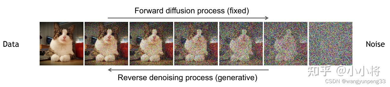
扩散模型包括两个过程：
前向过程（forward process）和反向过程（reverse process），其中前向过程又称为扩散过程（diffusion process），如下图所示。无论是前向过程还是反向过程都是一个参数化的马尔可夫链（Markov chain），其中反向过程可以用来生成数据，这里我们将通过变分推断来进行建模和求解

一、Loss计算

论文中的loss公式：

计算的是纯噪声 $\mathbf{ϵ}$ 和 ${\mathbf{ϵ}}_{\theta }\left(\sqrt{{\bar{\alpha }}_t}{\mathbf{x}}_0+\sqrt{1-{\bar{\alpha }}_t}\mathbf{ϵ},t\right)$ 之间的均方差：

noise = torch.randn_like(x_0)#其中noise的size是input_data一样的loss = F.mse_loss(self.model(x_t, t), noise, reduction='none')

计算 $x_t$：

$$x_t=\sqrt{{\bar{\alpha }}_t}{\mathbf{x}}_0+\sqrt{1-{\bar{\alpha }}_t}\mathbf{ϵ}$$

其中时刻信息 t 是通过 ${\bar{\alpha }}_t$ 表现的。
extract函数的作用是选取特定下标t的信息并转换成特定维度。
具体实现:

def extract(v, t, x_shape):"""Extract some coefficients at specified timesteps, then reshape to[batch_size, 1, 1, 1, 1, ...] for broadcasting purposes."""out = torch.gather(v, index=t, dim=0).float()return out.view([t.shape[0]] + [1] * (len(x_shape) - 1))       x_t = (extract(self.sqrt_alphas_bar, t, x_0.shape) * x_0 +extract(self.sqrt_one_minus_alphas_bar, t, x_0.shape) * noise)

计算 ${\bar{\alpha }}_t$

先根据${\beta }_1$和${\beta }_T$计算所有的${\beta }_t$

DDPM原始的论文设置的是线性增长，后面的论文有设置指数增长等其他方式。

 self.register_buffer('betas', torch.linspace(beta_1, beta_T, T).double())

再根据${\beta }_t$计算${\alpha }_t$
$${\alpha }_t=1-{\beta }_t$$

alphas = 1. - self.betas

累乘得到$\overline{{\alpha }_t}$

alphas_bar = torch.cumprod(alphas, dim=0)

最后将这些写入buffer

      self.register_buffer('sqrt_alphas_bar', torch.sqrt(alphas_bar))self.register_buffer('sqrt_one_minus_alphas_bar', torch.sqrt(1. - alphas_bar))

将$x_t$，t 输入到神经网络得到预测噪声 ${\mathbf{ϵ}}_{\theta }$ ,再根据公式不断采样得到$x_0$

self.register_buffer('posterior_log_var_clipped',torch.log(torch.cat([self.posterior_var[1:2], self.posterior_var[1:]])))self.register_buffer('posterior_mean_coef1',torch.sqrt(alphas_bar_prev) * self.betas / (1. - alphas_bar))self.register_buffer('posterior_mean_coef2',torch.sqrt(alphas) * (1. - alphas_bar_prev) / (1. - alphas_bar))def predict_xstart_from_xprev(self, x_t, t, xprev):assert x_t.shape == xprev.shapereturn (  # (xprev - coef2*x_t) / coef1extract(1. / self.posterior_mean_coef1, t, x_t.shape) * xprev -extract(self.posterior_mean_coef2 / self.posterior_mean_coef1, t,x_t.shape) * x_t

二、训练目标和采样目标

正向过程

正向过程即p过程，逆向过程即q过程、采样过程。

正向过程不涉及参数分布的计算和预测，可以理解为一个单纯add noise的过程。

训练和采样的训练目标如下：

class GaussianDiffusionTrainer(nn.Module):def __init__(self, model, beta_1, beta_T, T):super().__init__()self.model = modelself.T = Tself.register_buffer('betas', torch.linspace(beta_1, beta_T, T).double())alphas = 1. - self.betasalphas_bar = torch.cumprod(alphas, dim=0)# calculations for diffusion q(x_t | x_{t-1}) and othersself.register_buffer('sqrt_alphas_bar', torch.sqrt(alphas_bar))self.register_buffer('sqrt_one_minus_alphas_bar', torch.sqrt(1. - alphas_bar))def forward(self, x_0):"""Algorithm 1."""t = torch.randint(self.T, size=(x_0.shape[0], ), device=x_0.device)noise = torch.randn_like(x_0)x_t = (extract(self.sqrt_alphas_bar, t, x_0.shape) * x_0 +extract(self.sqrt_one_minus_alphas_bar, t, x_0.shape) * noise)loss = F.mse_loss(self.model(x_t, t), noise, reduction='none')return loss

逆向过程

$x_t$ 的分布符合高斯分布，这是通过均值和方差进行计算的：

计算 ${\sigma }_t\mathbf{Z}$ 使用：

torch.exp(0.5 * log_var) * noise

重点是计算这里的均值：
我们输入 $x_t$ , 得到 $x_{t-1}$

Alg1+Alg2 完整代码：

class GaussianDiffusionSampler(nn.Module):def __init__(self, model, beta_1, beta_T, T, img_size=32,mean_type='eps', var_type='fixedlarge'):assert mean_type in ['xprev' 'xstart', 'epsilon']assert var_type in ['fixedlarge', 'fixedsmall']super().__init__()self.model = modelself.T = Tself.img_size = img_sizeself.mean_type = mean_typeself.var_type = var_typeself.register_buffer('betas', torch.linspace(beta_1, beta_T, T).double())alphas = 1. - self.betasalphas_bar = torch.cumprod(alphas, dim=0)alphas_bar_prev = F.pad(alphas_bar, [1, 0], value=1)[:T]# calculations for diffusion q(x_t | x_{t-1}) and othersself.register_buffer('sqrt_recip_alphas_bar', torch.sqrt(1. / alphas_bar))self.register_buffer('sqrt_recipm1_alphas_bar', torch.sqrt(1. / alphas_bar - 1))# calculations for posterior q(x_{t-1} | x_t, x_0)self.register_buffer('posterior_var',self.betas * (1. - alphas_bar_prev) / (1. - alphas_bar))# below: log calculation clipped because the posterior variance is 0 at# the beginning of the diffusion chainself.register_buffer('posterior_log_var_clipped',torch.log(torch.cat([self.posterior_var[1:2], self.posterior_var[1:]])))self.register_buffer('posterior_mean_coef1',torch.sqrt(alphas_bar_prev) * self.betas / (1. - alphas_bar))self.register_buffer('posterior_mean_coef2',torch.sqrt(alphas) * (1. - alphas_bar_prev) / (1. - alphas_bar))def q_mean_variance(self, x_0, x_t, t):"""Compute the mean and variance of the diffusion posteriorq(x_{t-1} | x_t, x_0)"""assert x_0.shape == x_t.shapeposterior_mean = (extract(self.posterior_mean_coef1, t, x_t.shape) * x_0 +extract(self.posterior_mean_coef2, t, x_t.shape) * x_t)posterior_log_var_clipped = extract(self.posterior_log_var_clipped, t, x_t.shape)return posterior_mean, posterior_log_var_clippeddef predict_xstart_from_eps(self, x_t, t, eps):assert x_t.shape == eps.shapereturn (extract(self.sqrt_recip_alphas_bar, t, x_t.shape) * x_t -extract(self.sqrt_recipm1_alphas_bar, t, x_t.shape) * eps)def predict_xstart_from_xprev(self, x_t, t, xprev):assert x_t.shape == xprev.shapereturn (  # (xprev - coef2*x_t) / coef1extract(1. / self.posterior_mean_coef1, t, x_t.shape) * xprev -extract(self.posterior_mean_coef2 / self.posterior_mean_coef1, t,x_t.shape) * x_t)def p_mean_variance(self, x_t, t):# below: only log_variance is used in the KL computationsmodel_log_var = {# for fixedlarge, we set the initial (log-)variance like so to# get a better decoder log likelihood'fixedlarge': torch.log(torch.cat([self.posterior_var[1:2],self.betas[1:]])),'fixedsmall': self.posterior_log_var_clipped,}[self.var_type]model_log_var = extract(model_log_var, t, x_t.shape)# Mean parameterizationif self.mean_type == 'xprev':       # the model predicts x_{t-1}x_prev = self.model(x_t, t)x_0 = self.predict_xstart_from_xprev(x_t, t, xprev=x_prev)model_mean = x_prevelif self.mean_type == 'xstart':    # the model predicts x_0x_0 = self.model(x_t, t)model_mean, _ = self.q_mean_variance(x_0, x_t, t)elif self.mean_type == 'epsilon':   # the model predicts epsiloneps = self.model(x_t, t)x_0 = self.predict_xstart_from_eps(x_t, t, eps=eps)model_mean, _ = self.q_mean_variance(x_0, x_t, t)else:raise NotImplementedError(self.mean_type)x_0 = torch.clip(x_0, -1., 1.)return model_mean, model_log_vardef forward(self, x_T):"""Algorithm 2."""x_t = x_Tfor time_step in reversed(range(self.T)):t = x_t.new_ones([x_T.shape[0], ], dtype=torch.long) * time_stepmean, log_var = self.p_mean_variance(x_t=x_t, t=t)# no noise when t == 0if time_step > 0:noise = torch.randn_like(x_t)else:noise = 0x_t = mean + torch.exp(0.5 * log_var) * noisex_0 = x_treturn torch.clip(x_0, -1, 1)

二、Unet结构

• Unet的生成能力在GANs中早已被证明
• 在之前Unet结构的基础上，加入了attention和PE，形成了DDPM特有的Unet结构

Positional Embedding融入共享参数信息。positional embedding是transformer中一个重要的组成部分。因为在transformer中不包含RNN和CNN，为了让模型利用序列的顺序，必须注入一些关于序列中记号的相对或绝对位置的信息。

##DDPM中的位置编码
self.positional_embedding = nn.Parameter(th.randn(embed_dim, spacial_dim ** 2 + 1) / embed_dim ** 0.5)
x = x + self.positional_embedding[None, :, :].to(x.dtype)  # NC(HW+1)

为此添加位置编码在编码器和解码器堆栈的底部。位置编码与嵌入具有相同的维数模型，因此可以将两者相加。位置编码可以是可学习的，也可以是固定的。

DDPM特有的Unet结构

import math
import torch
from torch import nn
from torch.nn import init
from torch.nn import functional as F
class Swish(nn.Module):def forward(self, x):return x * torch.sigmoid(x)
class TimeEmbedding(nn.Module):def __init__(self, T, d_model, dim):assert d_model % 2 == 0super().__init__()emb = torch.arange(0, d_model, step=2) / d_model * math.log(10000)emb = torch.exp(-emb)pos = torch.arange(T).float()emb = pos[:, None] * emb[None, :]assert list(emb.shape) == [T, d_model // 2]emb = torch.stack([torch.sin(emb), torch.cos(emb)], dim=-1)assert list(emb.shape) == [T, d_model // 2, 2]emb = emb.view(T, d_model)self.timembedding = nn.Sequential(nn.Embedding.from_pretrained(emb),nn.Linear(d_model, dim),Swish(),nn.Linear(dim, dim),)self.initialize()def initialize(self):for module in self.modules():if isinstance(module, nn.Linear):init.xavier_uniform_(module.weight)init.zeros_(module.bias)def forward(self, t):emb = self.timembedding(t)return emb
class DownSample(nn.Module):def __init__(self, in_ch):super().__init__()self.main = nn.Conv2d(in_ch, in_ch, 3, stride=2, padding=1)self.initialize()def initialize(self):init.xavier_uniform_(self.main.weight)init.zeros_(self.main.bias)def forward(self, x, temb):x = self.main(x)return x
class UpSample(nn.Module):def __init__(self, in_ch):super().__init__()self.main = nn.Conv2d(in_ch, in_ch, 3, stride=1, padding=1)self.initialize()def initialize(self):init.xavier_uniform_(self.main.weight)init.zeros_(self.main.bias)def forward(self, x, temb):_, _, H, W = x.shapex = F.interpolate(x, scale_factor=2, mode='nearest')x = self.main(x)return x
class AttnBlock(nn.Module):def __init__(self, in_ch):super().__init__()self.group_norm = nn.GroupNorm(32, in_ch)self.proj_q = nn.Conv2d(in_ch, in_ch, 1, stride=1, padding=0)self.proj_k = nn.Conv2d(in_ch, in_ch, 1, stride=1, padding=0)self.proj_v = nn.Conv2d(in_ch, in_ch, 1, stride=1, padding=0)self.proj = nn.Conv2d(in_ch, in_ch, 1, stride=1, padding=0)self.initialize()def initialize(self):for module in [self.proj_q, self.proj_k, self.proj_v, self.proj]:init.xavier_uniform_(module.weight)init.zeros_(module.bias)init.xavier_uniform_(self.proj.weight, gain=1e-5)def forward(self, x):B, C, H, W = x.shapeh = self.group_norm(x)q = self.proj_q(h)k = self.proj_k(h)v = self.proj_v(h)q = q.permute(0, 2, 3, 1).view(B, H * W, C)k = k.view(B, C, H * W)w = torch.bmm(q, k) * (int(C) ** (-0.5))assert list(w.shape) == [B, H * W, H * W]w = F.softmax(w, dim=-1)v = v.permute(0, 2, 3, 1).view(B, H * W, C)h = torch.bmm(w, v)assert list(h.shape) == [B, H * W, C]h = h.view(B, H, W, C).permute(0, 3, 1, 2)h = self.proj(h)return x + h
class ResBlock(nn.Module):def __init__(self, in_ch, out_ch, tdim, dropout, attn=False):super().__init__()self.block1 = nn.Sequential(nn.GroupNorm(32, in_ch),Swish(),nn.Conv2d(in_ch, out_ch, 3, stride=1, padding=1),)self.temb_proj = nn.Sequential(Swish(),nn.Linear(tdim, out_ch),)self.block2 = nn.Sequential(nn.GroupNorm(32, out_ch),Swish(),nn.Dropout(dropout),nn.Conv2d(out_ch, out_ch, 3, stride=1, padding=1),)if in_ch != out_ch:self.shortcut = nn.Conv2d(in_ch, out_ch, 1, stride=1, padding=0)else:self.shortcut = nn.Identity()if attn:self.attn = AttnBlock(out_ch)else:self.attn = nn.Identity()self.initialize()def initialize(self):for module in self.modules():if isinstance(module, (nn.Conv2d, nn.Linear)):init.xavier_uniform_(module.weight)init.zeros_(module.bias)init.xavier_uniform_(self.block2[-1].weight, gain=1e-5)def forward(self, x, temb):h = self.block1(x)h += self.temb_proj(temb)[:, :, None, None]h = self.block2(h)h = h + self.shortcut(x)h = self.attn(h)return h
class UNet(nn.Module):def __init__(self, T, ch, ch_mult, attn, num_res_blocks, dropout):super().__init__()assert all([i < len(ch_mult) for i in attn]), 'attn index out of bound'tdim = ch * 4self.time_embedding = TimeEmbedding(T, ch, tdim)self.head = nn.Conv2d(3, ch, kernel_size=3, stride=1, padding=1)self.downblocks = nn.ModuleList()chs = [ch]  # record output channel when dowmsample for upsamplenow_ch = chfor i, mult in enumerate(ch_mult):out_ch = ch * multfor _ in range(num_res_blocks):self.downblocks.append(ResBlock(in_ch=now_ch, out_ch=out_ch, tdim=tdim,dropout=dropout, attn=(i in attn)))now_ch = out_chchs.append(now_ch)if i != len(ch_mult) - 1:self.downblocks.append(DownSample(now_ch))chs.append(now_ch)self.middleblocks = nn.ModuleList([ResBlock(now_ch, now_ch, tdim, dropout, attn=True),ResBlock(now_ch, now_ch, tdim, dropout, attn=False),])self.upblocks = nn.ModuleList()for i, mult in reversed(list(enumerate(ch_mult))):out_ch = ch * multfor _ in range(num_res_blocks + 1):self.upblocks.append(ResBlock(in_ch=chs.pop() + now_ch, out_ch=out_ch, tdim=tdim,dropout=dropout, attn=(i in attn)))now_ch = out_chif i != 0:self.upblocks.append(UpSample(now_ch))assert len(chs) == 0self.tail = nn.Sequential(nn.GroupNorm(32, now_ch),Swish(),nn.Conv2d(now_ch, 3, 3, stride=1, padding=1))self.initialize()def initialize(self):init.xavier_uniform_(self.head.weight)init.zeros_(self.head.bias)init.xavier_uniform_(self.tail[-1].weight, gain=1e-5)init.zeros_(self.tail[-1].bias)def forward(self, x, t):# Timestep embeddingtemb = self.time_embedding(t)# Downsamplingh = self.head(x)hs = [h]for layer in self.downblocks:h = layer(h, temb)hs.append(h)# Middlefor layer in self.middleblocks:h = layer(h, temb)# Upsamplingfor layer in self.upblocks:if isinstance(layer, ResBlock):h = torch.cat([h, hs.pop()], dim=1)h = layer(h, temb)h = self.tail(h)assert len(hs) == 0return h
if __name__ == '__main__':batch_size = 8model = UNet(T=1000, ch=128, ch_mult=[1, 2, 2, 2], attn=[1],num_res_blocks=2, dropout=0.1)x = torch.randn(batch_size, 3, 32, 32)t = torch.randint(1000, (batch_size, ))y = model(x, t)

Unet结构：

ResBlock基础模块：
引入时间编码 t ，self-attention机制

---

总结

DDPM有一个致命的问题，就是运算量过大，采样时间过长，如何加速这个采样时间？后续DDIM针对这个问题提出非马尔科夫链的生成模型。

在DDPMS中，生成过程被定义为特定马尔可夫扩散过程的反向过程。 我们通过一类非马尔可夫扩散过程将DDPMS推广到具有相同训练目标的非马尔可夫扩散过程。 这些非马尔可夫过程可以对应于确定性的生成过程，从而产生更快地产生高质量样本的隐式模型。

生成学习的三元悖论

Diffusion Models和GANs结合

DENOISING DIFFUSION GANS 论文地址

在本文中，我们认为这些模型中的慢采样从根本上归因于去噪步骤中的高斯假设，这种假设只适用于小步长。 为了实现大步长的去噪，从而减少去噪的总步数，我们提出了用复多峰分布来建模去噪分布。 我们引入了去噪扩散生成对抗网络（去噪扩散网络），该网络使用多模态条件GAN对每个去噪步骤进行建模。

代码地址汇总

diffusion models beats gans onimage syntheisis：https://github.com/openai/guided-diffusion
improved denoise diffusion probabilistic models：https://github.com/openai/improved-diffusion
DDPM MNIST：https://github.com/abarankab/DDPM
DDPM官方代码(TPU版本)：https://github.com/hojonathanho/diffusion
pytorch cifar10：https://github.com/w86763777/pytorch-ddpm
DDPM官方版本pytorch实现：GitHub - lucidrains/denoising-diffusion-pytorch: Implementation of Denoising Diffusion Probabilistic Model in Pytorch