Ensemble Kalman filter集合卡尔曼滤波

在气象预测领域，很多时候，模型具有 $O (10 e 8)$ 以上的量级，如果使用传统的卡尔曼滤波，协方差矩阵的更新将是一个~ $10 e 22$ 量级的计算操作，因此传统的卡尔曼滤波并不适用。集合卡尔曼滤波（Ensemble Kalman filter）用sample covariance模拟原本的协方差矩阵，用一个小的多的量级的矩阵运算代替原本的协方差矩阵更新。集合卡尔曼滤波与粒子滤波有相通之处，集合卡尔曼滤波假设用来做模拟的ensembles符合高斯分布。

本文将通过一个应用EnKF进行定位的python实例来初探集合卡尔曼滤波的概念。

参考：
【1】Ensemble_Kalman_filtering P. L. Houtekamer Herschel L. Mitchell
【2】ensemble_kalman_filter.py

根据参考【1】，集合卡尔曼滤波的公式为：

equations
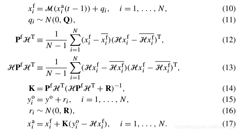
用通俗的话来解释参考【2】例子中的EnKF：对于机器人状态向量 $\theta,v]$ ，生成数量为N的ensembles，每一个ensemble都是机器人状态向量加上一个方差为 $Q$ 的误差，如此一来，通过上面的(12)(13)式我们可以看出，状态向量协方差矩阵 $P$ 已经不需要显式地计算出来了，我们只要针对每一个ensemble做计算就好了，而在现实问题中，ensemble的数量要远小于 $P$ 的维度，这就是集合卡尔曼滤波的精髓。

下面我们来看参考【2】中的代码：

for ip in range(NP):x = np.array([px[:, ip]]).T#  Predict with random input sampling# 预测：给输入加上方差为Q的随机误差：ud1 = u[0, 0] + np.random.randn() * Q[0, 0] ** 0.5ud2 = u[1, 0] + np.random.randn() * Q[1, 1] ** 0.5ud = np.array([[ud1, ud2]]).Tx = motion_model(x, ud)px[:, ip] = x[:, 0]

对应公式(10)，给运动模型的输入加上 $q_i$ ，计算每一个ensemble的状态向量的值。

接下来：

        # 根据状态预测值x和观测值z获取路标点加上观测方差R的空间位置z_posz_pos = observe_landmark_position(x, z)pz[:, ip] = z_pos[:, 0]

在这里我认为observe_landmark_position函数计算的其实是：

$Hx_i^f+r_i$

原因在计算(17)时会提到。

    x_ave = np.mean(px, axis=1)# 计算 x_f-x_f_barx_dif = px - np.tile(x_ave, (NP, 1)).Tz_ave = np.mean(pz, axis=1)# 计算 Hx_f-Hx_f_barz_dif = pz - np.tile(z_ave, (NP, 1)).TU = 1 / (NP - 1) * x_dif @ z_dif.TV = 1 / (NP - 1) * z_dif @ z_dif.T

接下来 $U$ 和 $V$ 我认为分别对应(12)(13)。在计算卡尔曼增益 $K$ 时，原代码直接计算：

K = U @ np.linalg.inv(V)

不知为什么好像没有体现出(14)式中的观测协方差 $R$ ，难道是因为我在上面提到的 $p z$ 中已经包含了观测噪声 $r$ ？

我对原代码进行了一些改动，加入了观测方差 $R$ （不能保证理论上的正确性），改动后的定位效果目测与原先没什么区别。

    # 以下是我的改动：# 观测协方差矩阵：R_a = np.diag([R[0,0]/2, R[0,0]/2] * z.shape[0])# 原代码：K = U @ np.linalg.inv(V)分母不包含观测协方差矩阵，# 这似乎与参考论文所述K的计算方法不符，不知道为什么这样处理# 在加入观测协方差R计算K后，与不加R计算K在定位结果上**目测**没有什么差别K = U @ np.linalg.inv(V + R_a)  # Kalman Gain

最后计算残差并进行更新：

    # 获取观测的真值：z_lm_pos = z[:, [2, 3]].reshape(-1, )# 更新：在这里pz包含了Hx_f和观测噪声rpx_hat = px + K @ (np.tile(z_lm_pos, (NP, 1)).T - pz)

在这里我们看到更新时直接用路标点真值减去了 $p z$ ，这也是为什么上面我提到observe_landmark_position函数计算的其实是 $Hx_i^f+r_i$

完整的包含注释的python代码如下：

"""Ensemble Kalman Filter(EnKF) localization sampleauthor: Ryohei Sasaki(rsasaki0109)modification: Junchuan ZhangRef:
Ensemble Kalman filtering
(https://rmets.onlinelibrary.wiley.com/doi/10.1256/qj.05.135)"""import mathimport matplotlib.pyplot as plt
import numpy as np
from scipy.spatial.transform import Rotation as Rot# 为了代码阅读上的方便，我在此加入了区别于simulation parameter的Q和R；
# Q和R数值上与simulation parameter一致（只是为了简化计算）
# 运动模型输入协方差：
Q = np.diag([1.0,np.deg2rad(30.0)]) ** 2  # predict state covariance
# 观测模型协方差：
R = np.diag([0.2, np.deg2rad(1.0)]) ** 2  # Observation covariance#  Simulation parameter
# 输入：
Q_sim = np.diag([1.0, np.deg2rad(30.0)]) ** 2
# 观测：
R_sim = np.diag([0.2, np.deg2rad(1.0)]) ** 2DT = 0.1  # time tick [s]
SIM_TIME = 50  # simulation time [s]
MAX_RANGE = 20.0  # maximum observation range# Ensemble Kalman filter parameter
# 很显然，增大NP，精度提高，计算量也随之提高
NP = 20  # Number of Particleshow_animation = Truedef calc_input():v = 1.0  # [m/s]yaw_rate = 0.1  # [rad/s]u = np.array([[v, yaw_rate]]).Treturn udef observation(xTrue, xd, u, RFID):xTrue = motion_model(xTrue, u)z = np.zeros((0, 4))for i in range(len(RFID[:, 0])):dx = RFID[i, 0] - xTrue[0, 0]dy = RFID[i, 1] - xTrue[1, 0]d = math.hypot(dx, dy)angle = pi_2_pi(math.atan2(dy, dx) - xTrue[2, 0])if d <= MAX_RANGE:dn = d + np.random.randn() * R_sim[0, 0] ** 0.5  # add noiseangle_with_noise = angle + np.random.randn() * R_sim[1, 1] ** 0.5# 在此将RFID的位置真值也一起放入了每组观测值内：zi = np.array([dn, angle_with_noise, RFID[i, 0], RFID[i, 1]])z = np.vstack((z, zi))# add noise to inputud = np.array([[u[0, 0] + np.random.randn() * Q_sim[0, 0] ** 0.5,u[1, 0] + np.random.randn() * Q_sim[1, 1] ** 0.5]]).Txd = motion_model(xd, ud)return xTrue, z, xd, uddef motion_model(x, u):F = np.array([[1.0, 0, 0, 0],[0, 1.0, 0, 0],[0, 0, 1.0, 0],[0, 0, 0, 0]])B = np.array([[DT * math.cos(x[2, 0]), 0],[DT * math.sin(x[2, 0]), 0],[0.0, DT],[1.0, 0.0]])x = F.dot(x) + B.dot(u)return xdef observe_landmark_position(x, landmarks):'''根据机器人空间位置x和路标点的观测值landmarks，计算加入观测噪声后的路标点空间值'''# landmark_pos大小为2倍路标点个数，因为将路标点x和y位置都放在了一个维度上：landmarks_pos = np.zeros((2 * landmarks.shape[0], 1))for (i, lm) in enumerate(landmarks):index = 2 * i# 在这里只包含R[0,0]，因为路标点x和y只涉及距离误差：q = R[0, 0] ** 0.5# 因此每一维加上sqrt(距离协方差/2)：landmarks_pos[index] = x[0, 0] + lm[0] * math.cos(x[2, 0] + lm[1]) + np.random.randn() * q / np.sqrt(2)landmarks_pos[index + 1] = x[1, 0] + lm[0] * math.sin(x[2, 0] + lm[1]) + np.random.randn() * q / np.sqrt(2)return landmarks_posdef calc_covariance(xEst, px):'''计算滤波更新后状态集合的方差'''cov = np.zeros((3, 3))for i in range(px.shape[1]):dx = (px[:, i] - xEst)[0:3]cov += dx.dot(dx.T)cov /= NPreturn covdef enkf_localization(px, z, u):"""Localization with Ensemble Kalman filterz: 前两位是观测，后两位是RFID的值u: 含有噪声的输入"""# print("________")pz = np.zeros((z.shape[0] * 2, NP))  # Particle store of zfor ip in range(NP):x = np.array([px[:, ip]]).T#  Predict with random input sampling# 预测：给输入加上方差为Q的随机误差：ud1 = u[0, 0] + np.random.randn() * Q[0, 0] ** 0.5ud2 = u[1, 0] + np.random.randn() * Q[1, 1] ** 0.5ud = np.array([[ud1, ud2]]).Tx = motion_model(x, ud)px[:, ip] = x[:, 0]# 根据状态预测值x和观测值z获取路标点加上观测方差R的空间位置z_posz_pos = observe_landmark_position(x, z)pz[:, ip] = z_pos[:, 0]x_ave = np.mean(px, axis=1)# 计算 x_f-x_f_barx_dif = px - np.tile(x_ave, (NP, 1)).Tz_ave = np.mean(pz, axis=1)# 计算 Hx_f-Hx_f_barz_dif = pz - np.tile(z_ave, (NP, 1)).TU = 1 / (NP - 1) * x_dif @ z_dif.TV = 1 / (NP - 1) * z_dif @ z_dif.T# 观测协方差矩阵：R_a = np.diag([R[0,0]/2, R[0,0]/2] * z.shape[0])# 原代码：K = U @ np.linalg.inv(V)分母不包含观测协方差矩阵，# 这似乎与参考论文所述K的计算方法不符，不知道为什么这样处理# 在加入观测协方差R计算K后，与不加R计算K在定位结果上**目测**没有什么差别K = U @ np.linalg.inv(V + R_a)  # Kalman Gain# 获取观测的真值：z_lm_pos = z[:, [2, 3]].reshape(-1, )# 更新：在这里pz包含了Hx_f和观测噪声rpx_hat = px + K @ (np.tile(z_lm_pos, (NP, 1)).T - pz)xEst = np.average(px_hat, axis=1).reshape(4, 1)# 这里的PEst只做画图之用，不参与预测-更新的迭代PEst = calc_covariance(xEst, px_hat)return xEst, PEst, px_hatdef plot_covariance_ellipse(xEst, PEst):  # pragma: no coverPxy = PEst[0:2, 0:2]eig_val, eig_vec = np.linalg.eig(Pxy)if eig_val[0] >= eig_val[1]:big_ind = 0small_ind = 1else:big_ind = 1small_ind = 0t = np.arange(0, 2 * math.pi + 0.1, 0.1)# eig_val[big_ind] or eiq_val[small_ind] were occasionally negative# numbers extremely close to 0 (~10^-20), catch these cases and set# the respective variable to 0try:a = math.sqrt(eig_val[big_ind])except ValueError:a = 0try:b = math.sqrt(eig_val[small_ind])except ValueError:b = 0x = [a * math.cos(it) for it in t]y = [b * math.sin(it) for it in t]angle = math.atan2(eig_vec[big_ind, 1], eig_vec[big_ind, 0])rot = Rot.from_euler('z', angle).as_matrix()[0:2, 0:2]fx = np.stack([x, y]).T @ rotpx = np.array(fx[:, 0] + xEst[0, 0]).flatten()py = np.array(fx[:, 1] + xEst[1, 0]).flatten()plt.plot(px, py, "--r")def pi_2_pi(angle):return (angle + math.pi) % (2 * math.pi) - math.pidef main():print(__file__ + " start!!")time = 0.0# RF_ID positions [x, y]RF_ID = np.array([[10.0, 0.0],[10.0, 10.0],[0.0, 15.0],[-5.0, 20.0]])# State Vector [x y yaw v]'xEst = np.zeros((4, 1))xTrue = np.zeros((4, 1))px = np.zeros((4, NP))  # Particle store of xxDR = np.zeros((4, 1))  # Dead reckoning# historyhxEst = xEsthxTrue = xTruehxDR = xTruewhile SIM_TIME >= time:time += DTu = calc_input()xTrue, z, xDR, ud = observation(xTrue, xDR, u, RF_ID)xEst, PEst, px = enkf_localization(px, z, ud)# store data historyhxEst = np.hstack((hxEst, xEst))hxDR = np.hstack((hxDR, xDR))hxTrue = np.hstack((hxTrue, xTrue))if show_animation:plt.cla()# for stopping simulation with the esc key.plt.gcf().canvas.mpl_connect('key_release_event',lambda event: [exit(0) if event.key == 'escape' else None])for i in range(len(z[:, 0])):plt.plot([xTrue[0, 0], z[i, 2]], [xTrue[1, 0], z[i, 3]], "-k")plt.plot(RF_ID[:, 0], RF_ID[:, 1], "*k")plt.plot(px[0, :], px[1, :], ".r")plt.plot(np.array(hxTrue[0, :]).flatten(),np.array(hxTrue[1, :]).flatten(), "-b")plt.plot(np.array(hxDR[0, :]).flatten(),np.array(hxDR[1, :]).flatten(), "-k")plt.plot(np.array(hxEst[0, :]).flatten(),np.array(hxEst[1, :]).flatten(), "-r")plot_covariance_ellipse(xEst, PEst)plt.axis("equal")plt.grid(True)plt.pause(0.001)if __name__ == '__main__':main()