Umap解决高维数据可视化的问题，以及高效降维。

Umap地址:https://github.com/lmcinnes/umap

文档地址：UMAP: Uniform Manifold Approximation and Projection for Dimension Reduction — umap 0.5 documentation

1.pip通过清华镜像安装方式：

pip install umap-learn[plot]  -i https://pypi.tuna.tsinghua.edu.cn/simple

2.使用方式

2.1连续性数据的可视化

# Umap的纯连续型数据降维与可视化
import numpy as np
from sklearn.datasets import fetch_california_housing
from sklearn.model_selection import train_test_split
from sklearn.preprocessing import StandardScaler
from sklearn.datasets import load_diabetes 
from sklearn.svm import SVR
import umap
import matplotlib.pyplot as plt
import seaborn as sns
import pandas as pd
%matplotlib inline

#  加载是数据集
load = load_diabetes()
data = pd.DataFrame(load.data)
data.columns = load.feature_names
target =  load.target

# 对特征数据进行标准化
scaled_data = StandardScaler().fit_transform(data)
# 使用umap对数据进行降维
embedding = umap.UMAP().fit_transform(scaled_data)
embedding.shape

 

# 对降维后的数据画图
plt.scatter(embedding[:, 0],embedding[:, 1])

 

 2.2对分类数据降维（含标签）

使用sklearn的手写数字来做数据可视化

# 分类手写数据的可视化
from sklearn.datasets import load_digits
digits = load_digits()

reducer = umap.UMAP(random_state=42)
reducer.fit(digits.data)
embedding = reducer.transform(digits.data)
# Verify that the result of calling transform is
# idenitical to accessing the embedding_ attribute
assert(np.all(embedding == reducer.embedding_))
embedding.shape

画图

plt.figure(figsize=(15,10))
plt.scatter(embedding[:, 0], embedding[:, 1], c=digits.target, cmap='Spectral', s=5)
plt.gca().set_aspect('equal', 'datalim')
plt.colorbar(boundaries=np.arange(11)-0.5).set_ticks(np.arange(10))
plt.title('UMAP projection of the Digits dataset', fontsize=24);

2.3对混合数据（离散、连续）在分别降维后组合在一起进行可视化

使用seaborn的钻石数据集

#####对混合数据（离散、连续）在分别降维后组合在一起进行可视化
# 砖石数据
from sklearn.preprocessing import RobustScaler
import umap.plot
diamonds = sns.load_dataset('diamonds')
diamonds.head()

price是标签，其余是特征

# 离散数据与连续数据的划分
numeric = diamonds[["carat", "table", "x", "y", "z"]].copy()
ordinal = diamonds[["cut", "color", "clarity"]].copy()
# 连续数据预处理
scaled_numeric = RobustScaler().fit_transform(numeric)
scaled_numeric[:5]# 离散数据数据因与顺序有关所以以数字划分表示等级
# 若离散数据与顺序无关，则使用独热编码后，UMAP设置参数metric为dice
ordinal["cut"] = ordinal.cut.map({"Fair":0, "Good":1, "Very Good":2, "Premium":3, "Ideal":4})
ordinal["color"] = ordinal.color.map({"D":0, "E":1, "F":2, "G":3, "H":4, "I":5, "J":6})
ordinal["clarity"] = ordinal.clarity.map({"I1":0, "SI2":1, "SI1":2, "VS2":3, "VS1":4, "VVS2":5, "VVS1":6, "IF":7})# 分别对数据进行降维，因分类数据与顺序有关所以设置参数为metric="manhattan"
numeric_mapper = umap.UMAP(n_neighbors=15, random_state=42).fit(scaled_numeric)
ordinal_mapper = umap.UMAP(metric="manhattan", n_neighbors=150, random_state=42).fit(ordinal.values)# 对连续数据进行画图，
umap.plot.points(numeric_mapper, values=diamonds["price"], cmap="viridis")

# 对分类数据分别画图
fig, ax = umap.plot.plt.subplots(2, 2, figsize=(12,12))
umap.plot.points(ordinal_mapper, labels=diamonds["color"], ax=ax[0,0])
umap.plot.points(ordinal_mapper, labels=diamonds["clarity"], ax=ax[0,1])
umap.plot.points(ordinal_mapper, labels=diamonds["cut"], ax=ax[1,0])
umap.plot.points(ordinal_mapper, values=diamonds["price"], cmap="viridis", ax=ax[1,1])

 

"""
这里有三种组合方式
那么，假设我们不能只是将原始数据粘合在一起并在其上贴上合理的指标，我们能做什么？ 
我们可以对模糊拓扑表示进行交集或并集。 还需要做一些工作来重申 UMAP 的理论假设（局部连通性，近似均匀分布）。 
幸运的是，只要您手头有适合的 UMAP 模型的副本（我们在这种情况下就是这样做的），UMAP 就可以使这相对容易。 
要使两个模型相交，只需使用 * 运算符； 使用 + 运算符来联合它们。
"""
intersection_mapper = numeric_mapper * ordinal_mapper
union_mapper = numeric_mapper + ordinal_mapper
contrast_mapper = numeric_mapper - ordinal_mapper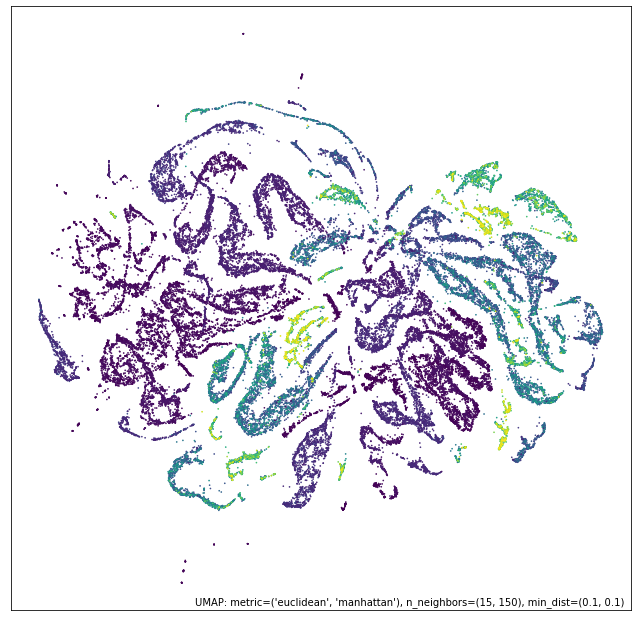

# 并集
umap.plot.points(union_mapper, labels=diamonds["color"])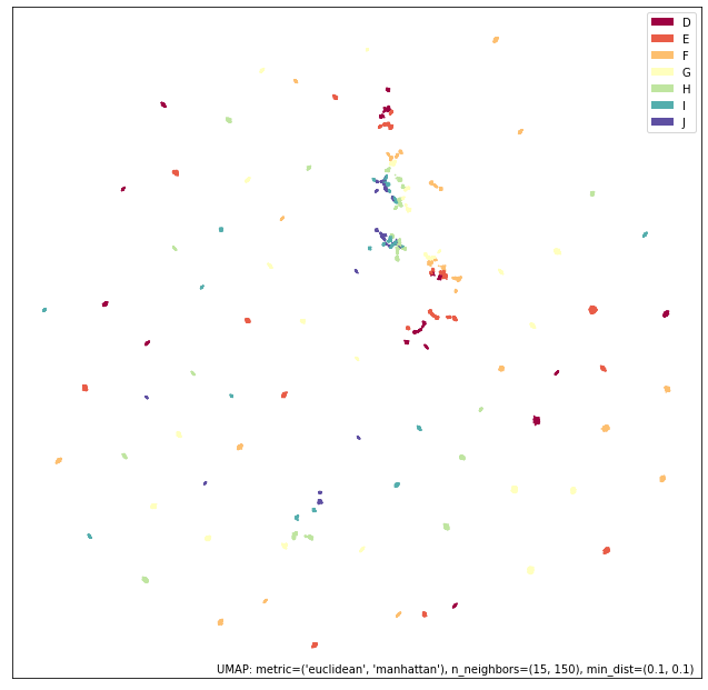

# 差集
umap.plot.points(contrast_mapper, values=diamonds["price"], cmap="viridis")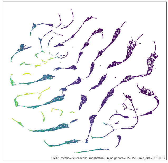

3.类的说明

class UMAP(BaseEstimator):"""Uniform Manifold Approximation and ProjectionFinds a low dimensional embedding of the data that approximatesan underlying manifold.Parameters----------n_neighbors: float (optional, default 15)The size of local neighborhood (in terms of number of neighboringsample points) used for manifold approximation. Larger valuesresult in more global views of the manifold, while smallervalues result in more local data being preserved. In generalvalues should be in the range 2 to 100.n_components: int (optional, default 2)The dimension of the space to embed into. This defaults to 2 toprovide easy visualization, but can reasonably be set to anyinteger value in the range 2 to 100.metric: string or function (optional, default 'euclidean')The metric to use to compute distances in high dimensional space.If a string is passed it must match a valid predefined metric. Ifa general metric is required a function that takes two 1d arrays andreturns a float can be provided. For performance purposes it isrequired that this be a numba jit'd function. Valid string metricsinclude:* euclidean* manhattan* chebyshev* minkowski* canberra* braycurtis* mahalanobis* wminkowski* seuclidean* cosine* correlation* haversine* hamming* jaccard* dice* russelrao* kulsinski* ll_dirichlet* hellinger* rogerstanimoto* sokalmichener* sokalsneath* yuleMetrics that take arguments (such as minkowski, mahalanobis etc.)can have arguments passed via the metric_kwds dictionary. At thistime care must be taken and dictionary elements must be orderedappropriately; this will hopefully be fixed in the future.n_epochs: int (optional, default None)The number of training epochs to be used in optimizing thelow dimensional embedding. Larger values result in more accurateembeddings. If None is specified a value will be selected based onthe size of the input dataset (200 for large datasets, 500 for small).learning_rate: float (optional, default 1.0)The initial learning rate for the embedding optimization.init: string (optional, default 'spectral')How to initialize the low dimensional embedding. Options are:* 'spectral': use a spectral embedding of the fuzzy 1-skeleton* 'random': assign initial embedding positions at random.* A numpy array of initial embedding positions.min_dist: float (optional, default 0.1)The effective minimum distance between embedded points. Smaller valueswill result in a more clustered/clumped embedding where nearby pointson the manifold are drawn closer together, while larger values willresult on a more even dispersal of points. The value should be setrelative to the ``spread`` value, which determines the scale at whichembedded points will be spread out.spread: float (optional, default 1.0)The effective scale of embedded points. In combination with ``min_dist``this determines how clustered/clumped the embedded points are.low_memory: bool (optional, default True)For some datasets the nearest neighbor computation can consume a lot ofmemory. If you find that UMAP is failing due to memory constraintsconsider setting this option to True. This approach is morecomputationally expensive, but avoids excessive memory use.set_op_mix_ratio: float (optional, default 1.0)Interpolate between (fuzzy) union and intersection as the set operationused to combine local fuzzy simplicial sets to obtain a global fuzzysimplicial sets. Both fuzzy set operations use the product t-norm.The value of this parameter should be between 0.0 and 1.0; a value of1.0 will use a pure fuzzy union, while 0.0 will use a pure fuzzyintersection.local_connectivity: int (optional, default 1)The local connectivity required -- i.e. the number of nearestneighbors that should be assumed to be connected at a local level.The higher this value the more connected the manifold becomeslocally. In practice this should be not more than the local intrinsicdimension of the manifold.repulsion_strength: float (optional, default 1.0)Weighting applied to negative samples in low dimensional embeddingoptimization. Values higher than one will result in greater weightbeing given to negative samples.negative_sample_rate: int (optional, default 5)The number of negative samples to select per positive samplein the optimization process. Increasing this value will resultin greater repulsive force being applied, greater optimizationcost, but slightly more accuracy.transform_queue_size: float (optional, default 4.0)For transform operations (embedding new points using a trained model_this will control how aggressively to search for nearest neighbors.Larger values will result in slower performance but more accuratenearest neighbor evaluation.a: float (optional, default None)More specific parameters controlling the embedding. If None thesevalues are set automatically as determined by ``min_dist`` and``spread``.b: float (optional, default None)More specific parameters controlling the embedding. If None thesevalues are set automatically as determined by ``min_dist`` and``spread``.random_state: int, RandomState instance or None, optional (default: None)If int, random_state is the seed used by the random number generator;If RandomState instance, random_state is the random number generator;If None, the random number generator is the RandomState instance usedby `np.random`.metric_kwds: dict (optional, default None)Arguments to pass on to the metric, such as the ``p`` value forMinkowski distance. If None then no arguments are passed on.angular_rp_forest: bool (optional, default False)Whether to use an angular random projection forest to initialisethe approximate nearest neighbor search. This can be faster, but ismostly on useful for metric that use an angular style distance suchas cosine, correlation etc. In the case of those metrics angular forestswill be chosen automatically.target_n_neighbors: int (optional, default -1)The number of nearest neighbors to use to construct the target simplcialset. If set to -1 use the ``n_neighbors`` value.target_metric: string or callable (optional, default 'categorical')The metric used to measure distance for a target array is using superviseddimension reduction. By default this is 'categorical' which will measuredistance in terms of whether categories match or are different. Furthermore,if semi-supervised is required target values of -1 will be trated asunlabelled under the 'categorical' metric. If the target array takescontinuous values (e.g. for a regression problem) then metric of 'l1'or 'l2' is probably more appropriate.target_metric_kwds: dict (optional, default None)Keyword argument to pass to the target metric when performingsupervised dimension reduction. If None then no arguments are passed on.target_weight: float (optional, default 0.5)weighting factor between data topology and target topology. A value of0.0 weights predominantly on data, a value of 1.0 places a strong emphasis ontarget. The default of 0.5 balances the weighting equally between data andtarget.transform_seed: int (optional, default 42)Random seed used for the stochastic aspects of the transform operation.This ensures consistency in transform operations.verbose: bool (optional, default False)Controls verbosity of logging.tqdm_kwds: dict (optional, defaul None)Key word arguments to be used by the tqdm progress bar.unique: bool (optional, default False)Controls if the rows of your data should be uniqued before beingembedded.  If you have more duplicates than you have n_neighbouryou can have the identical data points lying in different regions ofyour space.  It also violates the definition of a metric.For to map from internal structures back to your data use the variable_unique_inverse_.densmap: bool (optional, default False)Specifies whether the density-augmented objective of densMAPshould be used for optimization. Turning on this option generatesan embedding where the local densities are encouraged to be correlatedwith those in the original space. Parameters below with the prefix 'dens'further control the behavior of this extension.dens_lambda: float (optional, default 2.0)Controls the regularization weight of the density correlation termin densMAP. Higher values prioritize density preservation over theUMAP objective, and vice versa for values closer to zero. Setting thisparameter to zero is equivalent to running the original UMAP algorithm.dens_frac: float (optional, default 0.3)Controls the fraction of epochs (between 0 and 1) where thedensity-augmented objective is used in densMAP. The first(1 - dens_frac) fraction of epochs optimize the original UMAP objectivebefore introducing the density correlation term.dens_var_shift: float (optional, default 0.1)A small constant added to the variance of local radii in theembedding when calculating the density correlation objective toprevent numerical instability from dividing by a small numberoutput_dens: float (optional, default False)Determines whether the local radii of the final embedding (an inversemeasure of local density) are computed and returned in addition tothe embedding. If set to True, local radii of the original dataare also included in the output for comparison; the output is a tuple(embedding, original local radii, embedding local radii). This optioncan also be used when densmap=False to calculate the densities forUMAP embeddings.disconnection_distance: float (optional, default np.inf or maximal value for bounded distances)Disconnect any vertices of distance greater than or equal to disconnection_distance when approximating themanifold via our k-nn graph. This is particularly useful in the case that you have a bounded metric.  TheUMAP assumption that we have a connected manifold can be problematic when you have points that are maximallydifferent from all the rest of your data.  The connected manifold assumption will make such points have perfectsimilarity to a random set of other points.  Too many such points will artificially connect your space.precomputed_knn: tuple (optional, default (None,None,None))If the k-nearest neighbors of each point has already been calculated youcan pass them in here to save computation time. The number of nearestneighbors in the precomputed_knn must be greater or equal to then_neighbors parameter. This should be a tuple containing the outputof the nearest_neighbors() function or attributes from a previously fitUMAP object; (knn_indices, knn_dists,knn_search_index)."""

def points(umap_object,labels=None,values=None,theme=None,cmap="Blues",color_key=None,color_key_cmap="Spectral",background="white",width=800,height=800,show_legend=True,subset_points=None,ax=None,alpha=None,
):"""Plot an embedding as points. Currently this only worksfor 2D embeddings. While there are many optional parametersto further control and tailor the plotting, you need onlypass in the trained/fit umap model to get results. This plotutility will attempt to do the hard work of avoidingoverplotting issues, and make it easy to automaticallycolour points by a categorical labelling or numeric values.This method is intended to be used within a Jupyternotebook with ``%matplotlib inline``.Parameters----------umap_object: trained UMAP objectA trained UMAP object that has a 2D embedding.labels: array, shape (n_samples,) (optional, default None)An array of labels (assumed integer or categorical),one for each data sample.This will be used for coloring the points inthe plot according to their label. Note thatthis option is mutually exclusive to the ``values``option.values: array, shape (n_samples,) (optional, default None)An array of values (assumed float or continuous),one for each sample.This will be used for coloring the points inthe plot according to a colorscale associatedto the total range of values. Note that thisoption is mutually exclusive to the ``labels``option.theme: string (optional, default None)A color theme to use for plotting. A small set ofpredefined themes are provided which have relativelygood aesthetics. Available themes are:* 'blue'* 'red'* 'green'* 'inferno'* 'fire'* 'viridis'* 'darkblue'* 'darkred'* 'darkgreen'cmap: string (optional, default 'Blues')The name of a matplotlib colormap to use for coloringor shading points. If no labels or values are passedthis will be used for shading points according todensity (largely only of relevance for very largedatasets). If values are passed this will be used forshading according the value. Note that if themeis passed then this value will be overridden by thecorresponding option of the theme.color_key: dict or array, shape (n_categories) (optional, default None)A way to assign colors to categoricals. This can either bean explicit dict mapping labels to colors (as strings of form'#RRGGBB'), or an array like object providing one color foreach distinct category being provided in ``labels``. Eitherway this mapping will be used to color points according tothe label. Note that if themeis passed then this value will be overridden by thecorresponding option of the theme.color_key_cmap: string (optional, default 'Spectral')The name of a matplotlib colormap to use for categorical coloring.If an explicit ``color_key`` is not given a color mapping forcategories can be generated from the label list and selectinga matching list of colors from the given colormap. Notethat if themeis passed then this value will be overridden by thecorresponding option of the theme.background: string (optional, default 'white)The color of the background. Usually this will be either'white' or 'black', but any color name will work. Ideallyone wants to match this appropriately to the colors beingused for points etc. This is one of the things that themeshandle for you. Note that if themeis passed then this value will be overridden by thecorresponding option of the theme.width: int (optional, default 800)The desired width of the plot in pixels.height: int (optional, default 800)The desired height of the plot in pixelsshow_legend: bool (optional, default True)Whether to display a legend of the labelssubset_points: array, shape (n_samples,) (optional, default None)A way to select a subset of points based on an array of booleanvalues.ax: matplotlib axis (optional, default None)The matplotlib axis to draw the plot to, or if None, which isthe default, a new axis will be created and returned.alpha: float (optional, default: None)The alpha blending value, between 0 (transparent) and 1 (opaque).Returns-------result: matplotlib axisThe result is a matplotlib axis with the relevant plot displayed.If you are using a notebooks and have ``%matplotlib inline`` setthen this will simply display inline."""