我们通过一个demo(gan.py )来讲解对抗生成网络的原理和作用
1、创建真实数据
2、使用GAN训练噪声数据
3、通过1200次的训练使得生成的数据的分布跟真实数据的分布差不多
4、通过debug方式一步步的讲解
二、原理:
1、G(x)是生成的数据,放到判别D网络中,希望D网络输出 0;x是真实的输入,希望D网络输出 1

2、x输入G网络通过一系列的参数生成G(x)

3、对于D网络希望他的判别标准要高些,这样生成的数据才更能接近真实数据,这就需要D_pre网络进行预先的判断

三、代码实现的主要步骤:
1、构造判别网络模型 3–14
2、构造生成网络模型 15–32
3、构造损失函数 33–35
4、训练对抗生成网络
import argparse #1、参数解析的包
import numpy as np
from scipy.stats import norm
import tensorflow as tf
import matplotlib.pyplot as plt
from matplotlib import animation
import seaborn as sns #2、可视化的库sns.set(color_codes=True)  seed = 42
np.random.seed(seed)
tf.set_random_seed(seed)class DataDistribution(object):def __init__(self):self.mu = 4self.sigma = 0.5#44、def sample(self, N):samples = np.random.normal(self.mu, self.sigma, N)samples.sort()return samples#6、随机初始化分布,作为噪音点
class GeneratorDistribution(object):def __init__(self, range):self.range = rangedef sample(self, N):return np.linspace(-self.range, self.range, N) + \np.random.random(N) * 0.01#16、
def linear(input, output_dim, scope=None, stddev=1.0):#17、定义一个随机的初始化norm = tf.random_normal_initializer(stddev=stddev)#18、初始化常量为0const = tf.constant_initializer(0.0)with tf.variable_scope(scope or 'linear'):#19、w进行高斯处理话w = tf.get_variable('w', [input.get_shape()[1], output_dim], initializer=norm)#20、b进行常量初始化b = tf.get_variable('b', [output_dim], initializer=const)return tf.matmul(input, w) + b#29、生成网络只要两层就可以产生最终的输出结果
def generator(input, h_dim):h0 = tf.nn.softplus(linear(input, h_dim, 'g0'))h1 = linear(h0, 1, 'g1')return h1# 15、h0~h3 是分层的
def discriminator(input, h_dim):#h0是第一层的输出,h_dim * 2 隐层的数据h0 = tf.tanh(linear(input, h_dim * 2, 'd0'))h1 = tf.tanh(linear(h0, h_dim * 2, 'd1'))   h2 = tf.tanh(linear(h1, h_dim * 2, scope='d2'))#21、h3我们网络最总的输出结果h3 = tf.sigmoid(linear(h2, 1, scope='d3'))return h3
#24、优化器,学习率不断衰减的策略
def optimizer(loss, var_list, initial_learning_rate):decay = 0.95num_decay_steps = 150batch = tf.Variable(0)#25、学习率不断衰减的学习方式learning_rate = tf.train.exponential_decay(initial_learning_rate,batch,num_decay_steps,decay,staircase=True)#26、通过梯度下降定义求解器optimizer = tf.train.GradientDescentOptimizer(learning_rate).minimize(loss,global_step=batch,var_list=var_list)return optimizerclass GAN(object):#9、def __init__(self, data, gen, num_steps, batch_size, log_every):self.data = dataself.gen = genself.num_steps = num_stepsself.batch_size = batch_sizeself.log_every = log_everyself.mlp_hidden_size = 4self.learning_rate = 0.03#10、self._create_model()def _create_model(self):#11、构建D网络的骨架with tf.variable_scope('D_pre'):#12、输入,注意shape的参数self.pre_input = tf.placeholder(tf.float32, shape=(self.batch_size, 1))#13、labelself.pre_labels = tf.placeholder(tf.float32, shape=(self.batch_size, 1))#14、初始化操作D_pre = discriminator(self.pre_input, self.mlp_hidden_size)#22、预测值与真实值的差异D_pre和pre_labels的差异self.pre_loss = tf.reduce_mean(tf.square(D_pre - self.pre_labels))#23、self.pre_opt = optimizer(self.pre_loss, None, self.learning_rate)# This defines the generator network - it takes samples from a noise# distribution as input, and passes them through an MLP.with tf.variable_scope('Gen'):#27、噪音的输入self.z = tf.placeholder(tf.float32, shape=(self.batch_size, 1))#28、G网络用于数据的生成self.G = generator(self.z, self.mlp_hidden_size)# The discriminator tries to tell the difference between samples from the# true data distribution (self.x) and the generated samples (self.z).## Here we create two copies of the discriminator network (that share parameters),# as you cannot use the same network with different inputs in TensorFlow.with tf.variable_scope('Disc') as scope:#30、D网络用户判别功能self.x = tf.placeholder(tf.float32, shape=(self.batch_size, 1))#31、self.x 是真实的数据self.D1 = discriminator(self.x, self.mlp_hidden_size)scope.reuse_variables()#32、self.G是生成的数据self.D2 = discriminator(self.G, self.mlp_hidden_size)# Define the loss for discriminator and generator networks (see the original# paper for details), and create optimizers for both#33、判别网络的损失函数,希望D1趋近于1,希望D2趋近于0self.loss_d = tf.reduce_mean(-tf.log(self.D1) - tf.log(1 - self.D2))#34、生成网络(希望骗过判别网络)的损失函数,希望loss_g趋近于1self.loss_g = tf.reduce_mean(-tf.log(self.D2))self.d_pre_params = tf.get_collection(tf.GraphKeys.TRAINABLE_VARIABLES, scope='D_pre')self.d_params = tf.get_collection(tf.GraphKeys.TRAINABLE_VARIABLES, scope='Disc')self.g_params = tf.get_collection(tf.GraphKeys.TRAINABLE_VARIABLES, scope='Gen')#35、通过优化器不断地优化loss_d和loss_gself.opt_d = optimizer(self.loss_d, self.d_params, self.learning_rate)self.opt_g = optimizer(self.loss_g, self.g_params, self.learning_rate)#36、开始训练def train(self):with tf.Session() as session:tf.global_variables_initializer().run()# pretraining discriminatornum_pretrain_steps = 1000#37、先训练D-profor step in range(num_pretrain_steps):#38、d = (np.random.random(self.batch_size) - 0.5) * 10.0#39、labels = norm.pdf(d, loc=self.data.mu, scale=self.data.sigma)#40、迭代pretrain_loss, _ = session.run([self.pre_loss, self.pre_opt], {self.pre_input: np.reshape(d, (self.batch_size, 1)),self.pre_labels: np.reshape(labels, (self.batch_size, 1))})#41、self.weightsD = session.run(self.d_pre_params)# 42、copy weights from pre-training over to new D networkfor i, v in enumerate(self.d_params):session.run(v.assign(self.weightsD[i]))for step in range(self.num_steps):# 43、update discriminatorx = self.data.sample(self.batch_size)z = self.gen.sample(self.batch_size)loss_d, _ = session.run([self.loss_d, self.opt_d], {self.x: np.reshape(x, (self.batch_size, 1)),self.z: np.reshape(z, (self.batch_size, 1))})# 45、迭代优化两个网络 update generatorz = self.gen.sample(self.batch_size)loss_g, _ = session.run([self.loss_g, self.opt_g], {self.z: np.reshape(z, (self.batch_size, 1))})if step % self.log_every == 0:print('{}: {}\t{}'.format(step, loss_d, loss_g))                if step % 100 == 0 or step==0 or step == self.num_steps -1 :self._plot_distributions(session)def _samples(self, session, num_points=10000, num_bins=100):xs = np.linspace(-self.gen.range, self.gen.range, num_points)bins = np.linspace(-self.gen.range, self.gen.range, num_bins)# data distributiond = self.data.sample(num_points)pd, _ = np.histogram(d, bins=bins, density=True)# generated sampleszs = np.linspace(-self.gen.range, self.gen.range, num_points)g = np.zeros((num_points, 1))for i in range(num_points // self.batch_size):g[self.batch_size * i:self.batch_size * (i + 1)] = session.run(self.G, {self.z: np.reshape(zs[self.batch_size * i:self.batch_size * (i + 1)],(self.batch_size, 1))})pg, _ = np.histogram(g, bins=bins, density=True)return pd, pgdef _plot_distributions(self, session):pd, pg = self._samples(session)p_x = np.linspace(-self.gen.range, self.gen.range, len(pd))f, ax = plt.subplots(1)ax.set_ylim(0, 1)plt.plot(p_x, pd, label='real data')plt.plot(p_x, pg, label='generated data')plt.title('1D Generative Adversarial Network')plt.xlabel('Data values')plt.ylabel('Probability density')plt.legend()plt.show()
def main(args): #3、够造一个modelmodel = GAN(#4、参数DataDistribution(),#5、GeneratorDistribution(range=8),#7、定义参数args.num_steps,args.batch_size,#8、隔多长时间args.log_every,)model.train()def parse_args():parser = argparse.ArgumentParser()parser.add_argument('--num-steps', type=int, default=1200,help='the number of training steps to take')parser.add_argument('--batch-size', type=int, default=12,help='the batch size')parser.add_argument('--log-every', type=int, default=10,help='print loss after this many steps')return parser.parse_args()if __name__ == '__main__':main(parse_args())