Mean Shift聚类算法

1. 基本原理

对于Mean Shift算法，是一个迭代得步骤，即每次迭代的时候，都是找到圆里面点的平均位置作为新的圆心位置。说的简单一点，使得圆心一直往数据密集度最大的方向移动。
在这里插入图片描述

2. 基本的`Mean Shift`向量形式

对于给定的 $d$ 维空间 $R^d$ 中的 $n$ 个样本点 $x_i, i=1,2,...,n$ ，对于空间中的任意点 $x$ 的mean shift向量的基本形式可以表示为：
$M_h(x)=\frac {1}{k}\sum_{x_i \in S_h}(x_i-x)$
其中， $k$ 表示的是数据集中的点到 $x$ 小于球半径 $h$ 的数据点的个数， $S_h$ 是一个半径为 $h$ 的高维球区域， $S_h$ 的定义为：
$S_h(x)=(y|(y-x)(y-x)^T \leq h^2)$

这样的一种基本的Mean Shift形式存在一个问题：在 $S_h$ 区域内，每一个点对 $x$ 的贡献都是一样的，而实际上，这种贡献与 $x$ 到每一个点之间的距离是相关的，同时，对于每一个样本，其重要程度也不一样。

3. 改进的`Mean Shift`向量形式

假设在 $S_h$ 范围内，为了使得每一个样本点 $x_i$ 对于样本 $x$ 的贡献不一样，向基本的Mean Shift向量形式中增加核函数，得到如下的改进的Mean Shift向量形式：
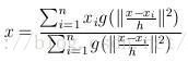
$M_h(x)=\frac {\sum_{x_i \in S_h}[K(\frac {x_i-x} {h})(x_i-x)]} {\sum_{x_i \in S_h}[K(\frac {x_i-x} {h})]}$
其中 $K(\frac {x_i-x} {h})$ 是高斯核函数，其函数形式如下：
$K(x_1,x_2)=K(\frac {x_1-x_2} {h})=\frac {1} {\sqrt {2\pi}h}e^{-\frac {(x_1-x_2)^2}{2h^2}}$
其中， $h$ 称为带宽bandwidth，即高维球区域 $S_h$ 的半径，不同带宽的核函数如下所示：
在这里插入图片描述

从图像可以看出，当带宽 $h$ 一定时，样本点之间的距离越近，其核函数的值越大；当样本点之间的距离相等时，随着高斯核函数的带宽 $h$ 的增大，核函数的值在减小

4. `Mean Shift`聚类流程

在未被标记的数据点中随机选择一个点作为中心center；
找出离center距离在bandwidth之内的所有点，记做集合 $M$ ，认为这些点属于簇 $c$ 。同时，把这些求内点属于这个类的概率加1，这个参数将用于最后步骤的分类
以center为中心点，计算从center开始到集合 $M$ 中每个元素的向量，将这些向量相加，得到向量shift
center = center+shift。即center沿着shift的方向移动，移动距离是||shift||
重复步骤2、3、4，直到shift的大小很小（就是迭代到收敛），记住此时的center。注意，这个迭代过程中遇到的点都应该归类到簇 $c$ 。
如果收敛时当前簇 $c$ 的center与其它已经存在的簇 $c_2$ 中心的距离小于阈值，那么把 $c_2$ 和 $c$ 合并。否则，把c作为新的聚类，增加1类。
重复1、2、3、4、5, 6直到所有的点都被标记访问
分类：根据每个类，对每个点的访问频率，取访问频率最大的那个类，作为当前点集的所属类。

5. 实例演示

import numpy as np 
import matplotlib.pyplot as plt from sklearn import cluster, datasets
from sklearn.preprocessing import StandardScalernp.random.seed(0)# 构建数据
n_samples = 1500
noisy_circles = datasets.make_circles(n_samples=n_samples, factor=0.5, noise=0.05)
noisy_moons = datasets.make_moons(n_samples=n_samples, noise=0.05)
blobs = datasets.make_blobs(n_samples=n_samples, random_state=8)data_sets = [(noisy_circles,{"quantile": 0.3}),(noisy_moons,{"quantile": 0.3}), (blobs, {"quantile": 0.3})
]
colors = ["#377eb8", "#ff7f00", "#4daf4a"]plt.figure(figsize=(15, 5))for i_dataset, (dataset, algo_params) in enumerate(data_sets):# 模型参数params = algo_params# 数据X, y = datasetX = StandardScaler().fit_transform(X)# 设置bandwidthbandwidth = cluster.estimate_bandwidth(X, quantile=params['quantile'])# 创建Mean Shiftms = cluster.MeanShift(bandwidth=bandwidth, bin_seeding=True)# 训练ms.fit(X)# 预测y_pred = ms.predict(X)y_pred_colors = []for i in y_pred:y_pred_colors.append(colors[i])plt.subplot(1, 3, i_dataset+1)plt.scatter(X[:, 0], X[:, 1], color=y_pred_colors)plt.show()