自动驾驶-MPC控制器

上节介绍了使用PID控制器控制车辆，PID控制器的优点是实现简单，处理速度快，但是缺点是不能处理有延迟的系统。本章介绍的MPC（modle predictive control）控制器能够很好的解决延迟的问题。

MPC控制器的和PID控制器一样，控制器输入包括车辆下一步的运行轨迹，车辆的当前状态，输出是航向角和加速度，用来控制方向盘，油门和刹车。不同之处在于，PID控制器是实时处理当前车辆与目标轨迹的差距来调整输出，使车辆接近目标轨迹，而MPC控制器将未来一个时间段 $t$ 分成 $N$ 个节点，预测每个节点的车辆状态，再调整控制器的输出使车辆尽可能接近参考轨迹。

MPC控制器的一般流程如下：

通过定位和地图模块得到当前路线，将这条路线离散化成一串坐标对，再拟合为三阶多项式；
根据车辆的当前位置和第一步生成的多项式系数预测未来一段时间车辆的行驶状态；
根据当前状态和预测状态的差异，调整航向角和加速度，使车辆状态接近预测状态；
重复以上三部。
其中第三步是MPC控制器的核心。

需要注意的是，调整航向角和加速度时，还要考虑乘车人的感受，所以要使加速度和航向角变化尽量平滑，下面详细介绍每一步的原理并给出代码实现。

拟合多项式

拟合多项式很好理解，就是把公路路线拟合称为一个三阶多项式，返回函数每一项系数。

// Fit a polynomial.
// Adapted from
// https://github.com/JuliaMath/Polynomials.jl/blob/master/src/Polynomials.jl#L676-L716
Eigen::VectorXd polyfit(Eigen::VectorXd xvals, Eigen::VectorXd yvals,int order) {assert(xvals.size() == yvals.size());assert(order >= 1 && order <= xvals.size() - 1);Eigen::MatrixXd A(xvals.size(), order + 1);for (int i = 0; i < xvals.size(); i++) {A(i, 0) = 1.0;}for (int j = 0; j < xvals.size(); j++) {for (int i = 0; i < order; i++) {A(j, i + 1) = A(j, i) * xvals(j);}}auto Q = A.householderQr();auto result = Q.solve(yvals);return result;
}

预测未来时间的行驶状态

有了上一步的多项式系数，就可以规划出未来一段时间内车辆的坐标位置，注意，地图给出的路线使用的是全剧坐标系，但是控制车辆是应该以车辆为中心，所以要进行坐标转换。

// Evaluate a polynomial.
double polyeval(Eigen::VectorXd coeffs, double x) {double result = 0.0;for (int i = 0; i < coeffs.size(); i++) {result += coeffs[i] * pow(x, i);}return result;
}Eigen::VectorXd roadside_x(ptsx.size());
Eigen::VectorXd roadside_y(ptsx.size());
vector<double> ptsx = j[1]["ptsx"];
vector<double> ptsy = j[1]["ptsy"];
double px = j[1]["x"];
double py = j[1]["y"];
double psi = j[1]["psi"];
double v = j[1]["speed"];double temp_x;
double temp_y;
// transform Descartes coordinates car space
for (size_t i = 0; i < ptsx.size(); i++) {temp_x = ptsx[i] - px;temp_y = ptsy[i] - py;roadside_y[i] = (temp_y * cos(psi) - temp_x * sin(psi));roadside_x[i] = (temp_y * sin(psi) + temp_x * cos(psi));
}
auto coeffs = polyfit(roadside_x, roadside_y, 3);

多项式可以计算未来若干时间节点车辆的目标位置，但是如何到达目标位置则是控制器的主要工作。

输出航向角和加速度

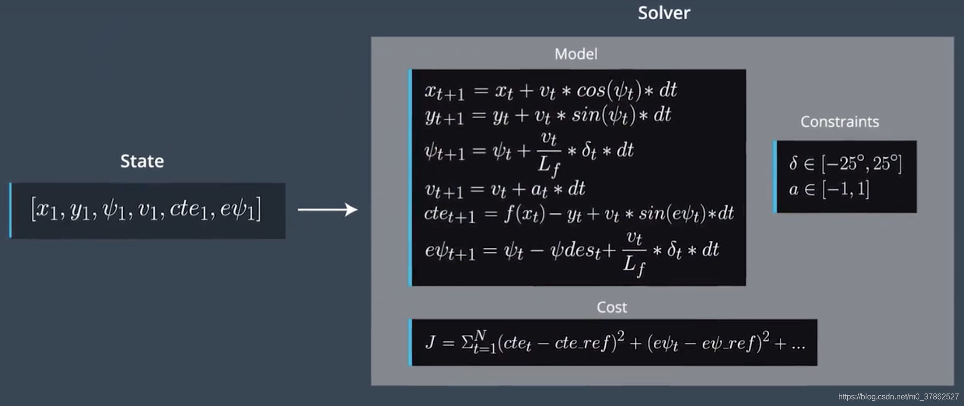
MPC控制器计算输出的过程可以看作一个工程最优化问题，即给出代价函数和约束条件，求解在约束条件下能使代价函数值最小的各个函数变量的最优值。
组成代价函数的变量包括位置的差异cte，航向角的差异epsi，速度差异，为了使乘车人感觉舒适，加速度和航向角速度也以及加速度行航向角速度的变化都不宜太高。
如下图所示，包括车辆的动态模型，代价函数和约束。动态模型用来预测接下来N个时间点车辆的状态，给出代价函数和约束条件，就可以将该模型转化为一个工程优化问题求解，最终目标是求解 $\psi和a$ ，即控制方向盘和油门或刹车，控制车辆按规划轨迹前进。
在这里插入图片描述
本章使用库函数cppad::ipopt::solve 求解工程最优化问题，其中f[0] 表示代价函数，f[1]~f[6N+1] 表示约束函数。

class FG_eval {public:// Fitted polynomial coefficientsEigen::VectorXd coeffs;FG_eval(Eigen::VectorXd coeffs) { this->coeffs = coeffs; }typedef CPPAD_TESTVECTOR(AD<double>) ADvector;void operator()(ADvector& fg, const ADvector& vars) {// TODO: implement MPC// `fg` a vector of the cost constraints, `vars` is a vector of variable values (state & actuators)// NOTE: You'll probably go back and forth between this function and// the Solver function below.fg[0] = 0;// Cost function// TODO: Define the cost related the reference state and// any anything you think may be beneficial.// The part of the cost based on the reference state.for (int t = 0; t < N; t++) {fg[0] += 10*CppAD::pow(vars[cte_start + t], 2);fg[0] += 100*CppAD::pow(vars[epsi_start + t], 2);fg[0] += CppAD::pow(vars[v_start + t] - ref_v, 2);}// Minimize the use of actuators.for (int t = 0; t < N - 1; t++) {fg[0] +=  CppAD::pow(vars[delta_start + t], 2);fg[0] +=  CppAD::pow(vars[a_start + t], 2);//fg[0] += 150*CppAD::pow(vars[delta_start + t] * vars[v_start+t],2);}// Minimize the value gap between sequential actuations.for (int t = 0; t < N - 2; t++) {fg[0] +=  10000*CppAD::pow(vars[delta_start + t + 1] - vars[delta_start + t], 2);fg[0] +=  CppAD::pow(vars[a_start + t + 1] - vars[a_start + t], 2);}fg[1 + px_start] = vars[px_start];fg[1 + py_start] = vars[py_start];fg[1 + psi_start] = vars[psi_start];fg[1 + v_start] = vars[v_start];fg[1 + cte_start] = vars[cte_start];fg[1 + epsi_start] = vars[epsi_start];for(int t = 1; t < N ; t++){// psi, v, delta at time tAD<double> psi0 = vars[psi_start + t - 1];AD<double> v0 = vars[v_start + t - 1];AD<double> delta0 = vars[delta_start + t - 1];// psi at time t+1AD<double> psi1 = vars[psi_start + t];// how psi changesfg[1 + psi_start + t] = psi1 - (psi0 - v0 * delta0 / Lf * dt);}for (int t = 1; t < N; t++) {// The state at time t+1 .AD<double> x1 = vars[px_start + t];AD<double> y1 = vars[py_start + t];AD<double> psi1 = vars[psi_start + t];AD<double> v1 = vars[v_start + t];AD<double> cte1 = vars[cte_start + t];AD<double> epsi1 = vars[epsi_start + t];// The state at time t.AD<double> x0 = vars[px_start + t - 1];AD<double> y0 = vars[py_start + t - 1];AD<double> psi0 = vars[psi_start + t - 1];AD<double> v0 = vars[v_start + t - 1];AD<double> cte0 = vars[cte_start + t - 1];AD<double> epsi0 = vars[epsi_start + t - 1];// Only consider the actuation at time t.AD<double> delta0 = vars[delta_start + t - 1];AD<double> a0 = vars[a_start + t - 1];if (t>1) {a0 = vars[a_start + t - 2];delta0 = vars[delta_start + t - 2];}AD<double> f0 = coeffs[0] + coeffs[1] * x0 + coeffs[2]* CppAD::pow(x0,2)+coeffs[3] * CppAD::pow(x0,3);AD<double> psides0 = CppAD::atan(coeffs[1]+ 2 * coeffs[2] * x0 + 3 * coeffs [3] * CppAD::pow(x0,2));// Here's `x` to get you started.// The idea here is to constraint this value to be 0.//// Recall the equations for the model:// x_[t] = x[t-1] + v[t-1] * cos(psi[t-1]) * dt// y_[t] = y[t-1] + v[t-1] * sin(psi[t-1]) * dt// psi_[t] = psi[t-1] + v[t-1] / Lf * delta[t-1] * dt// v_[t] = v[t-1] + a[t-1] * dt// cte[t] = f(x[t-1]) - y[t-1] + v[t-1] * sin(epsi[t-1]) * dt// epsi[t] = psi[t] - psides[t-1] + v[t-1] * delta[t-1] / Lf * dtfg[1 + px_start + t] = x1 - (x0 + v0 * CppAD::cos(psi0) * dt);fg[1 + py_start + t] = y1 - (y0 + v0 * CppAD::sin(psi0) * dt);fg[1 + psi_start + t] = psi1 - (psi0 - v0 * delta0 / Lf * dt);fg[1 + v_start + t] = v1 - (v0 + a0 * dt);fg[1 + cte_start + t] =cte1 - ((f0 - y0) + (v0 * CppAD::sin(epsi0) * dt));fg[1 + epsi_start + t] =epsi1 - ((psi0 - psides0) + v0 * delta0 / Lf * dt);}}
};
CppAD::vector<double> MPC::Solve(Eigen::VectorXd state, Eigen::VectorXd coeffs) {bool ok = true;size_t i;typedef CPPAD_TESTVECTOR(double) Dvector;// Set the number of model variables (includes both states and inputs).// For example: If the state is a 4 element vector, the actuators is a 2// element vector and there are 10 timesteps. The number of variables is://// 4 * 10 + 2 * 9size_t n_vars = 6 * N + (N - 1) * 2;//  Set the number of constraintssize_t n_constraints = 6 * N ;// Initial value of the independent variables.// SHOULD BE 0 besides initial state.Dvector vars(n_vars);for (i = 0; i < n_vars; i++) {vars[i] = 0;}vars[px_start] = state[0];vars[py_start] = state[1];vars[psi_start] = state[2];vars[v_start] = state[3];vars[cte_start] = state[4];vars[epsi_start] = state[5];Dvector vars_lowerbound(n_vars);Dvector vars_upperbound(n_vars);// Set lower and upper limits for variables.for (i = 0; i < delta_start; i++) {vars_lowerbound[i] = -1.0e10;vars_upperbound[i] = 1.0e10;}for (i = delta_start; i < a_start; i++) {vars_lowerbound[i] = -0.436;vars_upperbound[i] = 0.436;}for (i = a_start; i < n_vars; i++) {vars_lowerbound[i] = -1.0;vars_upperbound[i] = 1.0;}Dvector constraints_lowerbound(n_constraints);Dvector constraints_upperbound(n_constraints);for (i = 0; i < n_constraints; i++) {constraints_lowerbound[i] = 0;constraints_upperbound[i] = 0;}constraints_lowerbound[px_start] = state[0];constraints_upperbound[px_start] = state[0];constraints_lowerbound[py_start] = state[1];constraints_upperbound[py_start] = state[1];constraints_lowerbound[psi_start] = state[2];constraints_upperbound[psi_start] = state[2];constraints_lowerbound[v_start] = state[3];constraints_upperbound[v_start] = state[3];constraints_lowerbound[cte_start] = state[4];constraints_upperbound[cte_start] = state[4];constraints_lowerbound[epsi_start] = state[5];constraints_upperbound[epsi_start] = state[5];// Lower and upper limits for the constraints// Should be 0 besides initial state.// object that computes objective and constraintsFG_eval fg_eval(coeffs);//// NOTE: You don't have to worry about these options//// options for IPOPT solverstd::string options;// Uncomment this if you'd like more print informationoptions += "Integer print_level  0\n";// NOTE: Setting sparse to true allows the solver to take advantage// of sparse routines, this makes the computation MUCH FASTER. If you// can uncomment 1 of these and see if it makes a difference or not but// if you uncomment both the computation time should go up in orders of// magnitude.options += "Sparse  true        forward\n";options += "Sparse  true        reverse\n";// NOTE: Currently the solver has a maximum time limit of 0.5 seconds.// Change this as you see fit.options += "Numeric max_cpu_time          0.5\n";// place to return solutionCppAD::ipopt::solve_result<Dvector> solution;
#ifdef DEBUG// solve the problestd::cout<<"vars "<<vars<<std::endl;std::cout<<"vars_low"<<vars_lowerbound<<std::endl;std::cout<<"vars_upper"<<vars_upperbound<<std::endl;std::cout<<"cons_lower"<<constraints_lowerbound<<std::endl;std::cout<<"cons_upp"<<constraints_upperbound<<std::endl;
#endifCppAD::ipopt::solve<Dvector, FG_eval>(options, vars, vars_lowerbound, vars_upperbound, constraints_lowerbound,constraints_upperbound, fg_eval, solution);// Check some of the solution valuesok &= solution.status == CppAD::ipopt::solve_result<Dvector>::success;// Costdouble cost = solution.obj_value;std::cout << "Cost " << cost << std::endl;return solution.x;
}

完整代码请戳这里