趁着刚讲明白马上记录一下,不然以后又忘了_(:з」∠)_是一位老师给的现成的mpc小项目,代码写的很仔细能够帮助理解mpc的原理。
场景是一个二维平面的小车(看成一个质点),要运动到目标点,途中避开圆形范围的障碍物。
小车的矩形边框可以无视,只用作画图(方便展示旋转角度)。
MPC可以看做是一个算法,大概就是仿真系统运行K步,然后取第1步作为真实要走的步数。仿真通过常微分方程来计算,比如要仿真下一步step[k+1]=step[k]+ODE
第一步,因为有了ODE,又有了离散化的时间,我们就可以仿真出K步的位置。
第二步,设计目标函数。目标函数要最小,比如在这个例子中,就是距离goal的距离最短。一般是把K的距离都加起来再乘以一些参数啥的作为目标函数。
第三步,设置限制条件。比如速度不能超过多少,角速度不能超过多少,以及距离障碍物的距离要大于的半径等等。
这三样东西都有了呢,我们就可以把它们全部送进优化器里面,优化器会计算出来,优化的结果就放在state_predict数组里面,至于这个感觉还要研究一下语法的问题。

这个例子最后的效果如图:

%% Code for Nonlinear Model Predictive Control
% Status of cars and Navigation horizon can be modified in section
% "Set Robot Parameters" and "Set System Parameters".
% YALMIP required. Visit _yalmip.github.io_ for more information%% ============= Initialization =============
yalmip('clear'); clear ; close all; clc;%% ============= Render Obstacles =============
% Set number and size of obstacles
choice_size = 4;
choice_num = 1;
horizon = 15; % 仿真步数 15步if choice_num ~= 0obs = obs_render(choice_num,choice_size);
end%% ============= Set Robot Parameters =============
% Initialize robot status
robot = struct(...'length',4,...          % Length of the robot 画图用 后面三个点是换行用的,这样写好看'width',1.8,...         % Width of the robot 画图用'x_init',[-15;-15;0],...% Starting point of the robot 没用到'x_curr',[-15;-15;0],...% Current point of the robot 理论上初始化:x_curr=x_init,初始坐标和角度θ'x_goal',[15;15;0],...  % Goal point of the robot 目标坐标和角度θ'sample_freq',0.2,...   % Sampling frequency of the robot 步长,也可以说是时间间隔δt'flag',0,...            % Denote whether the robot has reached the goal point 标记是否到达目标'state_predict',0,...   % Predict sequence of state 预测的状态,里面应该存的是方程'control_predict',0);   % Predict sequence of control 控制的状态,里面应该存的是方程%% ============= Set System Parameters =============
% Set whether to print information for each optimization
verbose = 1;
% Global settings for map
world = struct(...'nx',3,...              % The number of parameters in state vector: q = [x y theta] 坐标和θ'nu',2,...              % The number of parameters in input vector: u = [v w] 速度和角速度'approx',0.3,...        % The range of error allowed near the goal point 'margin',20,...         % The margin of the world map'lim_v',2,...           % The limit of velosity'lim_w',pi/3,...        % The limit of angular velocity'horizon',horizon,...        % The prediction horizon 预测的步数 这里是15步'safety_distance',2.2); % The safety distance between two robots 这里只有一个robot 没用到%% ============= Initialize Map =============
% Plot initial and goal states
trace = init_plot_map(robot,world);% 画图用
if choice_num ~= 0plot_obs(obs,world,robot,'C');
end
fprintf('Press enter to continue.\n');pause% ============= Initialize Constraints and Objective =============
robot.control_predict = ...sdpvar(repmat(world.nu,1,world.horizon), repmat(1,1,world.horizon)); % 生成了1行15列的矩阵,里面的每个元素是三行1列[3,1]的sdpvar类型, 总的来说就是,3行15列的矩阵,用来存x,y,θ的,% sdqvar() 设置实型,intvar()设置整形,binvar()设置二进制形。
robot.state_predict = ...sdpvar(repmat(world.nx,1,world.horizon+1), repmat(1,1,world.horizon+1));% 生成了1行16列的矩阵,里面的每个元素是两行1列[2,1]的sdpvar类型, 总的来说就是,3行15列的矩阵,用来存 v,w的
constraints = [];
objective = 0;for k = 1:world.horizonrobot.state_predict{k+1} = robot.state_predict{k} + robot.sample_freq*...[cos(robot.state_predict{k}(3)) 0; sin(robot.state_predict{k}(3)) 0; 0 1]*...robot.control_predict{k};% 这是它的预测方程预测的方式是,下一步的速度是用当前步+从当前的x,y,θ出发,按照v,w的速度前行0.2步,得到下一步的状态(里面的x,y,xita,v,w都更新了)。objective = objective + (1+40*floor(k/world.horizon))*...((robot.state_predict{k+1}(1)-robot.x_goal(1))^2+...(robot.state_predict{k+1}(2)-robot.x_goal(2))^2+...(robot.state_predict{k+1}(3)-robot.x_goal(3))^2); %目标函数,floor是向下取整这里的方式是前面k-1步都值只+1,最后一步距离目标的位置会被考虑进来。constraints = [constraints,...-pi            <= robot.state_predict{k+1}(3) <= pi,...-world.lim_v   <= robot.control_predict{k}(1) <= world.lim_v,...-world.lim_w   <= robot.control_predict{k}(2) <= world.lim_w];% 限制条件,if choice_num ~= 0for cnt = 1:length(obs)bias_x = obs{cnt}.center(1);bias_y = obs{cnt}.center(2);min_dis = obs{cnt}.size + world.safety_distance;constraints = [constraints, (robot.state_predict{k+1}(1)-bias_x)^2+...(robot.state_predict{k+1}(2)-bias_y)^2>=min_dis^2]; % 障碍物的限制条件endend
end% ============= Solve optimization problem =============
step = 0;
time_cost = []; objective_val = []; predict_graph = [];while (robot.flag ~= 1)% Solve optimization problem and save calculation timet_start = cputime;optimize([constraints, robot.state_predict{1} == robot.x_curr], objective, ...sdpsettings('solver','fmincon','verbose',verbose)); % 送进优化器,优化应该是state_predict和control_predict一起优化的,运行完这句话以后,里面存的值应该都是使得当前目标函数取得最小值时候的状态。%也可以写成result = optimize() 判断result.problem==0 % 要去看看yalmip用法。robot.state_predict{1} == robot.x_curr 这个也加到了限制条件里面去,就相当于每次起步的初始状态赋值% v和w是我们需要控制的,所以不用初始值,每次都可以完全不一样,我们的优化目的就是找到最好的v和w使得 距离最近% v 和w 的限制也也在constraints 里面了。% sdpsettings是YALMIP和solver之间通信的桥梁,t_central = cputime - t_start;time_cost = [time_cost, t_central];objective_val = [objective_val, norm(robot.x_curr-robot.x_goal)];% Plot preduction statuspredict_graph = plot_predicted_states(predict_graph,world,robot);% Set and plot new current state% *** KNOWN PROBLEM ***% Handle possible buggy situations due to solver that the first input% might be zero. In such case, we choose the second predict state.robot.x_curr = value(robot.state_predict{2});if abs(value(robot.state_predict{1}) - value(robot.state_predict{2})) <= 0.01robot.x_curr = value(robot.state_predict{3});end% 这里第一步就是当前步,所以预测15步,取第二步作为真实的下一步,如果第二步和第一步差距很小,就采用第三步。plot_robot(robot.x_curr(1),robot.x_curr(2),robot.x_curr(3));% Determine whether reached the goal pointstep = step + 1; % step只是用来计步数if norm(robot.x_curr-robot.x_goal)<world.approx  %如果离终点小于阈值,就认为到达了robot.flag = 1;endpause(0.0001);
end
%后面就是画图啥的了
% Delete prediction status
for i = 1:length(predict_graph)% delete(predict_graph{i});
end% Directly display the information of time cost
disp(mean(time_cost));
disp(max(time_cost));%% ============= Save graph and data =============
% Generate plot of time consuming for each step
[time,obj] = plot_time_and_obj(time_cost,step,objective_val);
% Save graph and data as fig and mat files
file_id = ['nmpc_num_',num2str(choice_num),'_size_',num2str(choice_size)];
saveas(trace,['.\output\NMPC\trace_',file_id,'.fig']);
saveas(time,['.\output\NMPC\time_',file_id,'.fig']);
saveas(obj,['.\output\NMPC\obj_',file_id,'.fig']);
save(['.\output\NMPC\time_',file_id,'.mat'],'time_cost');
save(['.\output\NMPC\obj_',file_id,'.mat'],'objective_val');