文章目录
- 一、图示法
- (一)滞后图
- (二)自相关图
- (三)自相关图和偏自相关图
- 二 、DW检验法
- 三、Breusch-Godfrey检验
- (一)手动编制函数进行BG检验
- (二)调用statsmodels的函数进行BG检验
- 四、Ljung-Box检验
此文章首发于微信公众号:Python for Finance
链接:https://mp.weixin.qq.com/s/BuZg3hY8APHBr_vjmubn5g
多元线性回归模型的基本假设之一就是模型的随机干扰项相互独立或不相关。如果模型的随机干扰项违背了相互独立的基本假设,则称为存在序列相关性(自相关性)。
我们以伍德里奇《计量经济学导论:现代方法》的”第12章 时间序列回归中序列相关和异方差性“的案例12.4为例,使用BARIUM中的数据来进行序列相关性的检验。
import wooldridge as woo
import pandas as pd
import numpy as np
import statsmodels.api as sm
import statsmodels.formula.api as smfbarium = woo.dataWoo('barium')
T = len(barium)
barium.index = pd.date_range(start='1978-02', periods=T, freq='M')reg = smf.ols(formula='np.log(chnimp) ~ np.log(chempi) + np.log(gas) +''np.log(rtwex) + befile6 + affile6 + afdec6',data=barium)
results = reg.fit()
resid = results.resid#获取残差
一、图示法
由于残差 e t e_t et可以作为扰动项 u t u_t ut的估计,因此,如果存在序列相关性,必然会由残差项 e t e_t et反映出来,因此可利用 e t e_t et的变化图形来判断随机干扰项的序列相关性。
(一)滞后图
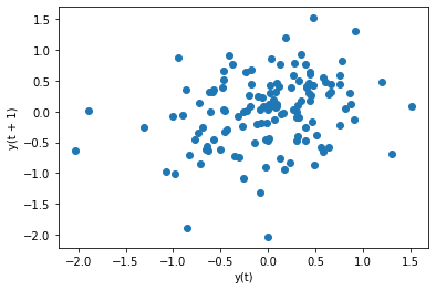
滞后图,就是将残差 e t e_t et和残差滞后n阶的散点图,需要用到pandas的lag_plot函数。
from pandas.plotting import lag_plot
lag_plot函数用法:
lag_plot(series, lag=1, ax=None, **kwds)
主要参数:
series :时间序列数据
lag : 滞后阶数,默认为1
ax : Matplotlib的子图对象,可选
我们绘制残差 e t e_t et和残差滞后1阶 e t − 1 e_{t-1} et−1的自相关图,代码如下:
lag_plot(resid, lag=1)
plt.show()
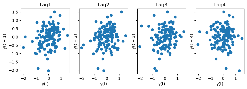
如果我们要绘制残差 e t e_t et与其滞后1-4阶的图,代码如下:
fig, axes = plt.subplots(1, 4, figsize=(10,3), sharex=True, sharey=True, dpi=100)#1行4列的画布
for i in range(4):lag_plot(resid,lag=i+1, ax=axes[i])axes[i].set_title(f'Lag{i+1}')
结果如下:
(二)自相关图
自相关图的绘制,可以使用pandas库的autocorrelation_plot函数
from pandas.plotting import autocorrelation_plot
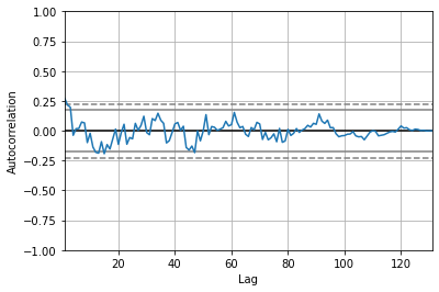
生成图片的横轴是滞后阶数,纵轴是自相关系数。
我们绘制残差项的自相关图,代码如下:
autocorrelation_plot(resid)
plt.show()
(三)自相关图和偏自相关图
自相关系数和偏自相关系数的区别
- 假设时间序列数据 y t y_t yt
- y t = α 0 + α 1 y t − 3 y_t=\alpha_0+\alpha_1y_{t-3} yt=α0+α1yt−3,这个 α 1 \alpha_1 α1就是, y t y_t yt和 y t − 3 y_{t-3} yt−3的自相关系数。
- y t = α 0 + α 1 y t − 1 + α 2 y t − 2 + α 3 y t − 3 y_t=\alpha_0+\alpha_1y_{t-1}+\alpha_2y_{t-2}+\alpha_3y_{t-3} yt=α0+α1yt−1+α2yt−2+α3yt−3,这个 α 3 \alpha_3 α3就是, y t y_t yt和 y t − 3 y_{t-3} yt−3的偏自相关系数。
自相关图和偏自相关图,建议使用statsmodels包的plot_acf, plot_pacf函数。
from statsmodels.graphics.tsaplots import plot_acf, plot_pacf #自相关图、偏自相关图
import matplotlib.pyplot as plt
plot_acf、plot_pacf函数的参数意义
plot_acf(x, ax=None, lags=None, *, alpha=0.05, use_vlines=True, adjusted=False, fft=False, missing='none', title='Autocorrelation', zero=True, auto_ylims=False, bartlett_confint=True, vlines_kwargs=None, **kwargs)
plot_pacf(x, ax=None, lags=None, alpha=0.05, method=None, use_vlines=True, title='Partial Autocorrelation', zero=True, vlines_kwargs=None, **kwargs)
x:一维的数据序列。
lags:滞后阶数,若未提供,则取np.arange(len(corr))
我们绘制残差项的自相关图,代码如下:
plot_acf(resid,lags=20) plt.show()
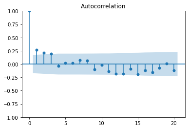
上图反映了resid序列的各阶自相关系数的大小,该图的高度值对应的是各阶自相关系数的值,蓝色区域是95%置信区间,这两条界线是检测自相关系数是否为0时所使用的判别标准:当代表自相关系数的柱条超过这两条界线时,可以认定自相关系数显著不为0。观察上图可知,1、2、3阶的自相关系数都在蓝色范围外,也就是落在了95%置信区间外,所以初步判断该序列可能存在短期的自相关性。
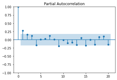
我们还可以绘制出残差项的偏自相关系数图,代码如下:
plot_pacf(resid,lags=20)
plt.show()
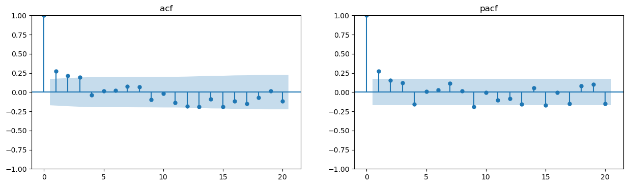
我们若希望将自相关系数图和偏自相关系数图合并成一张图,可以定义函数。
import matplotlib.pyplot as plt
def acf_pacf_plot(timeseries,lags):fig, axes = plt.subplots(nrows=1, ncols=2, figsize=(15, 4), dpi=100)plot_acf(timeseries, lags=lags,ax=axes[0])axes[0].set_title('acf') #设置自相关图标题,也可不设置,采用默认值Autocorrelationplot_pacf(timeseries,lags=lags,ax=axes[1])axes[1].set_title('pacf') #设置偏自相关图标题,也可不设置,采用默认值Partial Autocorrelationplt.show()
若我们需要对残差项做20阶的自相关图、偏自相关图,则调用上述函数即可,参数timeseries设置为resid,参数lags设置为20。
acf_pacf_plot(resid,20)
结果如下:
二 、DW检验法
DW检验是较早提出的自相关检验,现已不常用。它的主要缺点是只能检验一阶自相关,且必须在解释变量满足严格外生性的情况下才成立。
from statsmodels.stats.stattools import durbin_watson
print(f'D-W检验值为{durbin_watson(results.resid)}')
#返回结果:
D-W检验值为1.4584144308481417
三、Breusch-Godfrey检验
BG检验克服了DW检验的缺陷,适合于高阶序列相关及模型中存在滞后被解释变量的情形。
考虑如下多元线性模型:
y t = β 0 + β 1 x t 1 + β 2 x t 2 + . . . + β k x t k + u y_t=\beta_0+\beta_1x_{t1}+\beta_2x_{t2}+...+\beta_kx_{tk}+u yt=β0+β1xt1+β2xt2+...+βkxtk+u
若怀疑随机干扰项存在p阶序列相关:
u t = ρ 1 u t − 1 + ρ 2 u t − 2 + . . . + ρ p u t − p + ε t u_t=\rho_1u_{t-1}+\rho_2u_{t-2}+...+\rho_pu_{t-p}+\varepsilon_t ut=ρ1ut−1+ρ2ut−2+...+ρput−p+εt
检验原假设:
H 0 : ρ 1 = ρ 2 = . . . = ρ p = 0 H_0:\rho_1=\rho_2=...=\rho_p=0 H0:ρ1=ρ2=...=ρp=0
由于 u t u_t ut不可测,故用 e t e_t et替代,并引入解释变量,进行如下辅助回归:
e t = γ 1 x t 1 + γ 2 x t 2 + . . . + γ k x t k + δ 1 e t − 1 + δ 2 e t − 2 + . . . + δ p e t − p + ε t e_t=\gamma_1x_{t1}+\gamma_2x_{t2}+...+\gamma_kx_{tk}+\delta_1e_{t-1}+\delta_2e_{t-2}+...+\delta_pe_{t-p}+\varepsilon_t et=γ1xt1+γ2xt2+...+γkxtk+δ1et−1+δ2et−2+...+δpet−p+εt
无自相关的原假设相当于检验:
H 0 : γ 1 = γ 2 = . . . = γ p = 0 H_0:\gamma_1=\gamma_2=...=\gamma_p=0 H0:γ1=γ2=...=γp=0
BG检验的步骤:
(1)将 y t y_t yt对 x t 1 x_{t1} xt1, x t 2 x_{t2} xt2,…, x t k x_{tk} xtk做回归,求出OLS残差 e t e_t et
(2)将 e t e_t et对 x t 1 x_{t1} xt1, x t 2 x_{t2} xt2,…, x t k x_{tk} xtk, e t − 1 e_{t-1} et−1, e t − 2 e_{t-2} et−2,…, e t − p e_{t-p} et−p做回归
(3)计算 e t − 1 e_{t-1} et−1, e t − 2 e_{t-2} et−2,…, e t − p e_{t-p} et−p联合显著的F检验
(一)手动编制函数进行BG检验
barium['resid'] = results.resid
barium['resid_lag1'] = barium['resid'].shift(1)
barium['resid_lag2'] = barium['resid'].shift(2)
barium['resid_lag3'] = barium['resid'].shift(3)reg_manual = smf.ols(formula='resid~ np.log(chempi) + np.log(gas) +''np.log(rtwex) + befile6 + affile6 + afdec6+''resid_lag1 + resid_lag2 + resid_lag3', data=barium)
results_manual = reg_manual.fit()hypotheses = ['resid_lag1 = 0', 'resid_lag2 = 0', 'resid_lag3 = 0']
ftest_manual = results_manual.f_test(hypotheses)
F_statistic = ftest_manual.fvalue
F_pval = ftest_manual.pvalue
print(f'BG检验的F统计量: {F_statistic}')
print(f'BG检验的p值: {F_pval}')'''
BG检验的F统计量: 5.122907054069363
BG检验的p值: 0.0022898028329663344
'''
我们可以查看辅助回归的回归结果:
print(results_manual.summary())
'''OLS Regression Results
==============================================================================
Dep. Variable:                  resid   R-squared:                       0.116
Model:                            OLS   Adj. R-squared:                  0.048
Method:                 Least Squares   F-statistic:                     1.719
Date:                Sat, 14 May 2022   Prob (F-statistic):             0.0920
Time:                        09:28:33   Log-Likelihood:                -104.56
No. Observations:                 128   AIC:                             229.1
Df Residuals:                     118   BIC:                             257.6
Df Model:                           9
Covariance Type:            nonrobust
==================================================================================coef    std err          t      P>|t|      [0.025      0.975]
----------------------------------------------------------------------------------
Intercept        -14.3691     20.656     -0.696      0.488     -55.273      26.535
np.log(chempi)    -0.1432      0.472     -0.303      0.762      -1.078       0.792
np.log(gas)        0.6233      0.886      0.704      0.483      -1.131       2.378
np.log(rtwex)      0.1787      0.391      0.457      0.649      -0.596       0.953
befile6           -0.0859      0.251     -0.342      0.733      -0.583       0.411
affile6           -0.1221      0.255     -0.479      0.632      -0.626       0.382
afdec6            -0.0668      0.274     -0.244      0.808      -0.610       0.476
resid_lag1         0.2215      0.092      2.417      0.017       0.040       0.403
resid_lag2         0.1340      0.092      1.454      0.148      -0.048       0.317
resid_lag3         0.1255      0.091      1.378      0.171      -0.055       0.306
==============================================================================
Omnibus:                        6.375   Durbin-Watson:                   1.947
Prob(Omnibus):                  0.041   Jarque-Bera (JB):                5.978
Skew:                          -0.444   Prob(JB):                       0.0503
Kurtosis:                       3.576   Cond. No.                     9.78e+03
==============================================================================Notes:
[1] Standard Errors assume that the covariance matrix of the errors is correctly specified.
[2] The condition number is large, 9.78e+03. This might indicate that there are
strong multicollinearity or other numerical problems.
'''
由于辅助回归使用了 e t − p e_{t-p} et−p损失了p个样本观测值,故样本容量仅有 ( n − p ) (n-p) (n−p)。Davidson and MacKinnon(1993)建议,把残差中因滞后而缺失的项用其期望值0来代替,以保持样本容量为n。
则代码修改为:
barium['resid'] = results.resid
barium['resid_lag1'] = barium['resid'].shift(1).fillna(0) #将残差缺失项用0来代替
barium['resid_lag2'] = barium['resid'].shift(2).fillna(0) #将残差缺失项用0来代替
barium['resid_lag3'] = barium['resid'].shift(3).fillna(0) #将残差缺失项用0来代替reg_manual = smf.ols(formula='resid~ np.log(chempi) + np.log(gas) +''np.log(rtwex) + befile6 + affile6 + afdec6+''resid_lag1 + resid_lag2 + resid_lag3', data=barium)
results_manual = reg_manual.fit()hypotheses = ['resid_lag1 = 0', 'resid_lag2 = 0', 'resid_lag3 = 0']
ftest_manual = results_manual.f_test(hypotheses)
F_statistic = ftest_manual.fvalue
F_pval = ftest_manual.pvalue
print(f'BG检验的F统计量: {F_statistic}')
print(f'BG检验的p值: {F_pval}')'''
BG检验的F统计量: 5.124662239772509
BG检验的p值: 0.002263719767131574
'''
我们可以查看辅助回归的回归结果:
print(results_manual.summary())
'''OLS Regression Results
==============================================================================
Dep. Variable:                  resid   R-squared:                       0.113
Model:                            OLS   Adj. R-squared:                  0.047
Method:                 Least Squares   F-statistic:                     1.708
Date:                Sat, 14 May 2022   Prob (F-statistic):             0.0942
Time:                        09:26:57   Log-Likelihood:                -106.95
No. Observations:                 131   AIC:                             233.9
Df Residuals:                     121   BIC:                             262.7
Df Model:                           9
Covariance Type:            nonrobust
==================================================================================coef    std err          t      P>|t|      [0.025      0.975]
----------------------------------------------------------------------------------
Intercept        -13.1407     20.351     -0.646      0.520     -53.431      27.149
np.log(chempi)    -0.0435      0.457     -0.095      0.924      -0.948       0.862
np.log(gas)        0.5436      0.876      0.621      0.536      -1.190       2.277
np.log(rtwex)      0.2024      0.386      0.525      0.601      -0.561       0.966
befile6           -0.0815      0.251     -0.325      0.746      -0.578       0.415
affile6           -0.1243      0.254     -0.489      0.626      -0.628       0.379
afdec6            -0.0776      0.274     -0.283      0.777      -0.619       0.464
resid_lag1         0.2186      0.090      2.416      0.017       0.039       0.398
resid_lag2         0.1341      0.092      1.458      0.147      -0.048       0.316
resid_lag3         0.1257      0.091      1.381      0.170      -0.054       0.306
==============================================================================
Omnibus:                        5.672   Durbin-Watson:                   1.955
Prob(Omnibus):                  0.059   Jarque-Bera (JB):                5.196
Skew:                          -0.414   Prob(JB):                       0.0744
Kurtosis:                       3.516   Cond. No.                     9.76e+03
==============================================================================Notes:
[1] Standard Errors assume that the covariance matrix of the errors is correctly specified.
[2] The condition number is large, 9.76e+03. This might indicate that there are
strong multicollinearity or other numerical problems.
'''
(二)调用statsmodels的函数进行BG检验
从statsmodels库的stats子模块的diagnostic工具中导入acorr_breusch_godfrey
from statsmodels.stats.diagnostic import acorr_breusch_godfrey #BG检验
acorr_breusch_godfrey函数的参数意义及返回结果
acorr_breusch_godfrey(res, nlags=None, store=False)
参数介绍:
res : 回归结果,对该模型的残差进行自相关检验。
nlags : 滞后阶数
store : 默认为False;若为True,则会返回ResultsStore返回值:
lm : LM统计量值
lm_pvalue : LM统计量的p值,若p值小于显著性水平,则拒绝无自相关性的原假设,即存在自相关性
fvalue : F统计量值
f_pvalue : F统计量对应的p值,若p值小于显著性水平,则拒绝无自相关性的原假设,即存在自相关性
res_store:ResultsStore,若store为True则返回
Davidson and MacKinnon(1993)建议,把残差中因滞后而缺失的项用其期望值0来代替,以保持样本容量为n。acorr_breusch_godfrey函数采用的是Davidson-MacKinnon方法。
对上述模型做BG检验,代码如下:
bg_result = acorr_breusch_godfrey(results,nlags=3)
bg_lm_statistic = bg_result[0]
bg_lm_pval = bg_result[1]
bg_F_statistic= bg_result[2]
bg_F_pval = bg_result[3]
bg_test_output=pd.Series(bg_result[0:4],index=['bg_lm_statistic','bg_lm_pval','bg_F_statistic','bg_F_pval'])
print(bg_test_output)'''
bg_lm_statistic    14.768156
bg_lm_pval          0.002026
bg_F_statistic      5.124662
bg_F_pval           0.002264
dtype: float64
'''
同时,我们可以查看BG检验的辅助回归模型结果:
print(bg_result[4].resols.summary())
'''OLS Regression Results
==============================================================================
Dep. Variable:                      y   R-squared:                       0.113
Model:                            OLS   Adj. R-squared:                  0.047
Method:                 Least Squares   F-statistic:                     1.708
Date:                Fri, 13 May 2022   Prob (F-statistic):             0.0942
Time:                        20:26:10   Log-Likelihood:                -106.95
No. Observations:                 131   AIC:                             233.9
Df Residuals:                     121   BIC:                             262.7
Df Model:                           9
Covariance Type:            nonrobust
==============================================================================coef    std err          t      P>|t|      [0.025      0.975]
------------------------------------------------------------------------------
const         -6.5703     10.175     -0.646      0.520     -26.715      13.575
x1            -0.0435      0.457     -0.095      0.924      -0.948       0.862
x2             0.5436      0.876      0.621      0.536      -1.190       2.277
x3             0.2024      0.386      0.525      0.601      -0.561       0.966
x4            -0.0815      0.251     -0.325      0.746      -0.578       0.415
x5            -0.1243      0.254     -0.489      0.626      -0.628       0.379
x6            -0.0776      0.274     -0.283      0.777      -0.619       0.464
x7            -6.5703     10.175     -0.646      0.520     -26.715      13.575
x8             0.2186      0.090      2.416      0.017       0.039       0.398
x9             0.1341      0.092      1.458      0.147      -0.048       0.316
x10            0.1257      0.091      1.381      0.170      -0.054       0.306
==============================================================================
Omnibus:                        5.672   Durbin-Watson:                   1.955
Prob(Omnibus):                  0.059   Jarque-Bera (JB):                5.196
Skew:                          -0.414   Prob(JB):                       0.0744
Kurtosis:                       3.516   Cond. No.                     7.48e+16
==============================================================================Notes:
[1] Standard Errors assume that the covariance matrix of the errors is correctly specified.
[2] The smallest eigenvalue is 1.33e-29. This might indicate that there are
strong multicollinearity problems or that the design matrix is singular.
'''
acorr_breusch_godfrey函数做辅助回归的因变量为残差项,自变量为[1,A,1,B],其中A为解释变量,B为残差滞后项。
在以上回归结果中,y代表残差项,x1-x6代表解释变量,x8-x10代表残差滞后项,(const+x7)代表常数项。
我们可以在acorr_breusch_godfrey函数的基础上,编制一个能返回自相关性检验结果的函数。
def bg_test(results,nlags):bg_result = acorr_breusch_godfrey(results,nlags=3) bg_lm_statistic = bg_result[0]bg_lm_pval = bg_result[1]bg_F_statistic= bg_result[2] bg_F_pval = bg_result[3]bg_test_output=pd.Series(bg_result[0:4],index=['bg_lm_statistic','bg_lm_pval','bg_F_statistic','bg_F_pval']) return bg_test_output
#失败,先放着。同时,我们可以编制一个函数,可以
p_value_threshold=0.1
autocorrelation_results = pd.DataFrame(columns=['Autocorrelation test', 'lag', 'p-value', 'outcome']
for i in range(0, 5):lag=i+1bg_F_pval = acorr_breusch_godfrey(results, nlags=lag)[3]autocorrelation_results.iloc[i] = ['Breusch-Godfrey', lag, bg_F_pval, 'Pass' if bg_F_pval> p_value_threshold else 'Fail']
四、Ljung-Box检验
LB检验:
- H0假设:序列的每个值是独立的,即纯随机
- HA假设:序列之间不是独立的,即存在相关性
从statsmodels库的stats子模块的diagnostic工具中导入acorr_ljungbox
from statsmodels.stats.diagnostic import acorr_ljungbox #LB检验
acorr_ljungbox函数的参数意义及返回结果
acorr_ljungbox(x, lags=None, boxpierce=False, model_df=0, period=None, return_df=True, auto_lag=False)
y : 一维的数据序列
lags:滞后阶数,若lags为整数,则会对[1,lags]区间的所有滞后阶数做LB检验;若lags为列表,则只展示列表内的滞后阶数的LB检验结果。
boxpierce:默认False,为True时表示除返回LB统计量还会返回Box和Pierce的Q统计量返回结果为:
lbvalue: Ljung-Box检验统计量
pvalue: Ljung-Box检验统计量对应的p值,若p值小于显著性水平,则拒绝纯随机序列的原假设,即序列不是纯随机序列
bpvalue:Box-Pierce检验统计量
bppvalue: Box-Pierce检验统计量对应的p值,若p值小于显著性水平,则拒绝纯随机序列的原假设
对上述模型做LB检验,代码如下:
print(acorr_ljungbox(results.resid, lags=[10])) #对10阶做LB检验
'''lb_stat  lb_pvalue
10  24.445298   0.006502
'''
print(acorr_ljungbox(results.resid, lags=10)) #对1-10阶均做LB检验
'''lb_stat  lb_pvalue
1    9.821711   0.001725
2   16.072867   0.000323
3   21.332651   0.000090
4   21.532752   0.000248
5   21.571232   0.000632
6   21.619047   0.001419
7   22.365714   0.002197
8   22.973536   0.003398
9   24.381012   0.003738
10  24.445298   0.006502
'''
LB检验的p值小于0.01, 则拒绝纯随机序列的原假设,即序列不是纯随机序列。
参考文献:
Python时间序列分析https://www.machinelearningplus.com/time-series/time-series-analysis-python/
Python与时间序列https://blog.csdn.net/yuanzhoulvpi/article/details/120384708