---

前言

Canny边缘检测是一种非常流行的边缘检测算法，是John Canny在1986年提出的。它是一个多阶段的算法，即由多个步骤构成。本文主要讲解了Canny算子的原理及实现过程。

---

一、Canny的实现步骤

通常情况下边缘检测的目的是在保留原有图像属性的情况下，显著减少图像的数据规模。有多种算法可以进行边缘检测，虽然Canny算法年代久远，但可以说它是边缘检测的一种标准算法，而且仍在研究中广泛使用。

1. 应用高斯滤波来平滑图像，目的是去除噪声
2. 找寻图像的强度梯度（intensity gradients）
3. 应用非最大抑制（non-maximum suppression）技术来消除边误检（本来不是但检测出来是）
4. 应用双阈值的方法来决定可能的（潜在的）边界
5. 利用滞后技术来跟踪边界

二、具体实现

1.高斯平滑滤波

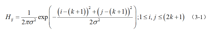
滤波是为了去除噪声，选用高斯滤波也是因为在众多噪声滤波器中，高斯表现最好（表现怎么定义的？最好好到什么程度？），你也可以试试其他滤波器如均值滤波、中值滤波等等。一个大小为(2k+1)x(2k+1)的高斯滤波器核（核一般都是奇数尺寸的）的生成方程式由下式给出：

下面是手动创建一个高斯滤波核的函数：

def gaussian_kernel(size, sigma):""" Implementation of Gaussian Kernel.This function follows the gaussian kernel formula,and creates a kernel matrix.Hints:- Use np.pi and np.exp to compute pi and exp.Args:size: int of the size of output matrix.sigma: float of sigma to calculate kernel.Returns:kernel: numpy array of shape (size, size)."""kernel = np.zeros((size, size))### YOUR CODE HEREfor x in range(size):for y in range(size):kernel[x, y] = 1 / (2*np.pi*sigma*sigma) * np.exp(-(x*x+y*y)/(2*sigma*sigma))### END YOUR CODEreturn kernel

这是定义卷积计算过程的函数：

def conv(image, kernel):""" An implementation of convolution filter.This function uses element-wise multiplication and np.sum()to efficiently compute weighted sum of neighborhood at eachpixel.Args:image: numpy array of shape (Hi, Wi).kernel: numpy array of shape (Hk, Wk).Returns:out: numpy array of shape (Hi, Wi)."""Hi, Wi = image.shapeHk, Wk = kernel.shapeout = np.zeros((Hi, Wi))# For this assignment, we will use edge values to pad the images.# Zero padding will make derivatives at the image boundary very big,# whereas we want to ignore the edges at the boundary.pad_width0 = Hk // 2pad_width1 = Wk // 2pad_width = ((pad_width0,pad_width0),(pad_width1,pad_width1))padded = np.pad(image, pad_width, mode='edge')### YOUR CODE HEREx = Hk // 2y = Wk // 2# 横向遍历卷积后的图像for i in range(pad_width0, Hi-pad_width0): # 纵向遍历卷积后的图像for j in range(pad_width1, Wi-pad_width1): split_img = image[i-pad_width0:i+pad_width0+1, j-pad_width1:j+pad_width1+1]# 对应元素相乘out[i, j] = np.sum(np.multiply(split_img, kernel))# out = (out-out.min()) * (1/(out.max()-out.min()) * 255).astype('uint8')### END YOUR CODEreturn out

接下来就是用自己写的高斯滤波卷积核去卷原来的图片：

# Test with different kernel_size and sigma
kernel_size = 5
sigma = 1.4# Load image
img = io.imread('iguana.png', as_gray=True)# Define 5x5 Gaussian kernel with std = sigma
kernel = gaussian_kernel(kernel_size, sigma)# Convolve image with kernel to achieve smoothed effect
smoothed = conv(img, kernel)plt.subplot(1,2,1)
plt.imshow(img)
plt.title('Original image')
plt.axis('off')plt.subplot(1,2,2)
plt.imshow(smoothed)
plt.title('Smoothed image')
plt.axis('off')plt.show()

结果是下面两张图片，可以看到图像的边缘被明显地模糊了，图像的抗噪能力变强了。

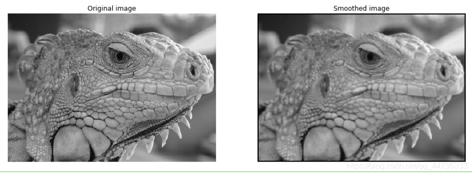
总结一下这一步：高斯滤波其实就是将所指像素用周围的像素的某种均值代替(即卷积核)，卷积核尺寸越大，去噪能力越强，因此噪声越少，但图片越模糊，canny检测算法抗噪声能力越强，但模糊的副作用也会导致定位精度不高。
高斯的卷积核大小推荐：一般情况下，尺寸5 * 5，3 * 3也行。

2.计算梯度大小和方向

对于一张图片来说，梯度能很好地反映其像素的变化情况，而梯度变化越大，说明相邻像素之间存在着较大差异，放大到整张图片来说，就是在某一块区域存在边缘，从视觉上来说就是用黑到白(灰度图片读入)。
梯度的计算分为大小和方向，首先需要求出各个方向上的梯度，然后求平方根和切线。
以下是x、y方向上梯度的计算方式：

代码实现：

def partial_x(img):""" Computes partial x-derivative of input img.Hints:- You may use the conv function in defined in this file.Args:img: numpy array of shape (H, W).Returns:out: x-derivative image."""out = None### YOUR CODE HERE# 对x求偏导kernel = np.array(([-1, 0, 1], [-1, 0, 1], [-1, 0, 1]))# np.random.randint(10, size=(3, 3))out = conv(img, kernel) / 2### END YOUR CODEreturn outdef partial_y(img):""" Computes partial y-derivative of input img.Hints:- You may use the conv function in defined in this file.Args:img: numpy array of shape (H, W).Returns:out: y-derivative image."""out = None### YOUR CODE HERE# 对y求偏导kernel = np.array(([1, 1, 1], [0, 0, 0], [-1, -1, -1]))# np.random.randint(10, size=(3, 3))out = conv(img, kernel) / 2### END YOUR CODEreturn outdef gradient(img):""" Returns gradient magnitude and direction of input img.Args:img: Grayscale image. Numpy array of shape (H, W).Returns:G: Magnitude of gradient at each pixel in img.Numpy array of shape (H, W).theta: Direction(in degrees, 0 <= theta < 360) of gradientat each pixel in img. Numpy array of shape (H, W).Hints:- Use np.sqrt and np.arctan2 to calculate square root and arctan"""G = np.zeros(img.shape)theta = np.zeros(img.shape)### YOUR CODE HEREGx = partial_x(img)Gy = partial_y(img)# 求梯度的大小(平方和的根号)G = np.sqrt(np.power(Gx, 2) + np.power(Gy, 2))theta = np.arctan2(Gy, Gx) * 180 / np.pi # 转换成角度制### END YOUR CODEreturn G, theta

可以拿一张图片来测试一下：

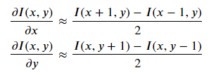
# Compute partial derivatives of smoothed image
Gx = partial_x(smoothed)
Gy = partial_y(smoothed)plt.subplot(1,2,1)
plt.imshow(Gx)
plt.title('Derivative in x direction')
plt.axis('off')plt.subplot(1,2,2)
plt.imshow(Gy)
plt.title('Derivative in y direction')
plt.axis('off')plt.show()

可以看到，[-1, 0, 1], [-1, 0, 1], [-1, 0, 1]对应了x方向上的边缘检测(在碰到x方向垂直的边界的时候计算出来的数值更大，所以像素更亮)，[1, 1, 1], [0, 0, 0], [-1, -1, -1]同理对应了y方向上的边缘检测。
另外有45°和135°的边缘检测，我这里没有着手去实现，如果有兴趣可以去尝试一下，就是会出现不同方向上的边缘。

3.非极大抑制

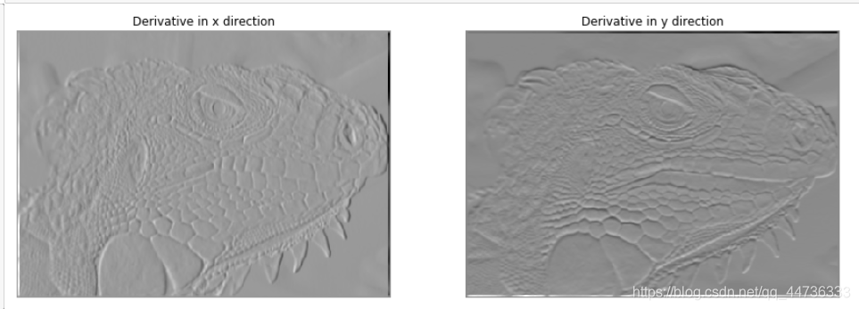
用sobel算子或者是其他简单的边缘检测方法，计算出来的边缘太粗了，就是说原本的一条边用几条几乎重叠的边所代替了，导致视觉上看起来边界很粗。非极大抑制是一种瘦边经典算法。它抑制那些梯度不够大的像素点，只保留最大的梯度，从而达到瘦边的目的。
a) 将其梯度方向近似为以下值中的一个[0,45,90,135,180,225,270,315]（即上下左右和45度方向）这一步是为了方便使用梯度；
b) 比较该像素点，和其梯度方向正负方向的像素点的梯度强度，这里比较的范围一般为像素点的八邻域；
c) 如果该像素点梯度强度最大则保留，否则抑制(删除，即置为0)；

可以看到经过非极大抑制后，图像的边缘明显变细了，边界显得更加清晰了。
代码附上：

def non_maximum_suppression(G, theta):""" Performs non-maximum suppression.This function performs non-maximum suppression along the directionof gradient (theta) on the gradient magnitude image (G).Args:G: gradient magnitude image with shape of (H, W).theta: direction of gradients with shape of (H, W).Returns:out: non-maxima suppressed image."""H, W = G.shapeout = np.zeros((H, W))# 将角度近似到45°的对角线, 正负无所谓, 只看对角线跟水平垂直# Round the gradient direction to the nearest 45 degreestheta = np.floor((theta + 22.5) / 45) * 45### BEGIN YOUR CODEanchor = np.stack(np.where(G!=0)).T  # 获取非零梯度的位置    for x, y in anchor:center_point = G[x, y]current_theta = theta[x, y]dTmp1 = 0dTmp2 = 0W = 0if current_theta >= 0 and current_theta < 45:g1, g2, g3, g4 = G[x + 1, y - 1], G[x + 1, y], G[x - 1, y + 1], G[x - 1, y]W = abs(np.tan(current_theta*np.pi/180))  # tan0-45范围为0-1dTmp1 = W * g1 + (1-W) * g2dTmp2 = W * g3 + (1-W) * g4elif current_theta >= 45 and current_theta < 90:g1, g2, g3, g4 = G[x+1, y-1], G[x, y-1], G[x-1, y+1], G[x, y+1]W = abs(np.tan((current_theta-90)*np.pi/180))dTmp1 = W * g1 + (1-W) * g2dTmp2 = W * g3 + (1-W) * g4elif current_theta >= -90 and current_theta < -45:g1, g2, g3, g4 = G[x-1, y-1], G[x, y-1], G[x+1, y+1], G[x, y+1]W = abs(np.tan((current_theta-90)*np.pi/180))dTmp1 = W * g1 + (1-W) * g2dTmp2 = W * g3 + (1-W) * g4elif current_theta>=-45 and current_theta<0:g1, g2, g3, g4 = G[x+1, y+1], G[x+1, y], G[x-1, y-1], G[x-1, y]W = abs(np.tan(current_theta * np.pi / 180))dTmp1 = W * g1 + (1-W) * g2dTmp2 = W * g3 + (1-W) * g4if dTmp1 < center_point and dTmp2 < center_point:   out[x,y]=center_pointreturn out

4.双阈值(Double Thresholding)和滞后边界跟踪

经过非极大抑制后图像中仍然有很多噪声点。Canny算法中应用了一种叫双阈值的技术。
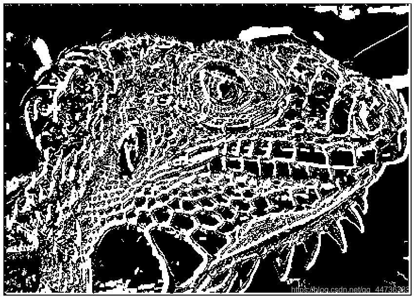
即设定一个阈值上界和阈值下界（opencv中通常由人为指定的），图像中的像素点如果大于阈值上界则认为必然是边界（称为强边界，strong edge），小于阈值下界则认为必然不是边界，两者之间的则认为是候选项（称为弱边界，weak edge），需进行进一步处理。我查阅资料，了解到上界一般是下界的2-3倍，实现出来的效果比较好。

上图中，左边的是经过上界筛选的强边界，即肯定是边界；右边的是结果是强边界加上0.5权重的弱边界所呈现的效果(展示弱边界没有啥意义)。可以看到相较于之前的非极大抑制，双阈值的算法很大程度上提取到了真正的边界(但是对于不同的图片有不同的阈值参数)。
代码附上：

def double_thresholding(img, high, low):"""Args:img: numpy array of shape (H, W) representing NMS edge response.high: high threshold(float) for strong edges.low: low threshold(float) for weak edges.Returns:strong_edges: Boolean array representing strong edges.Strong edeges are the pixels with the values greater thanthe higher threshold.weak_edges: Boolean array representing weak edges.Weak edges are the pixels with the values smaller or equal to thehigher threshold and greater than the lower threshold."""strong_edges = np.zeros(img.shape, dtype=np.bool)weak_edges = np.zeros(img.shape, dtype=np.bool)### YOUR CODE HEREH, W = img.shapefor i in range(0, H):for j in range(0, W):if img[i, j] > high:strong_edges[i, j] = Trueelif img[i, j] >= low:weak_edges[i, j] = True### END YOUR CODEreturn strong_edges, weak_edges

可以肯定的是，强边缘必然是边缘点，因此必须将T1设置的足够高，以要求像素点的梯度值足够大（变化足够剧烈），而弱边缘可能是边缘，也可能是噪声，如何判断呢？当弱边缘的周围8邻域有强边缘点存在时，就将该弱边缘点变成强边缘点，以此来实现对强边缘的补充。

滞后边界跟踪(对弱边缘的二次判断)，代码如下：

def get_neighbors(y, x, H, W):""" Return indices of valid neighbors of (y, x).Return indices of all the valid neighbors of (y, x) in an array ofshape (H, W). An index (i, j) of a valid neighbor should satisfythe following:1. i >= 0 and i < H2. j >= 0 and j < W3. (i, j) != (y, x)Args:y, x: location of the pixel.H, W: size of the image.Returns:neighbors: list of indices of neighboring pixels [(i, j)]."""neighbors = []for i in (y-1, y, y+1):for j in (x-1, x, x+1):if i >= 0 and i < H and j >= 0 and j < W:if (i == y and j == x):continueneighbors.append((i, j))return neighborsdef link_edges(strong_edges, weak_edges):""" Find weak edges connected to strong edges and link them.Iterate over each pixel in strong_edges and perform breadth firstsearch across the connected pixels in weak_edges to link them.Here we consider a pixel (a, b) is connected to a pixel (c, d)if (a, b) is one of the eight neighboring pixels of (c, d).Args:strong_edges: binary image of shape (H, W).weak_edges: binary image of shape (H, W).Returns:edges: numpy boolean array of shape(H, W)."""H, W = strong_edges.shape# 获取强边界的非零元素坐标，一行为一组坐标indices = np.stack(np.nonzero(strong_edges)).Tprint(indices)edges = np.zeros((H, W), dtype=np.bool)# Make new instances of arguments to leave the original# references intactweak_edges = np.copy(weak_edges)edges = np.copy(strong_edges)### YOUR CODE HEREfor (x, y) in indices:neighbors = get_neighbors(x, y, H, W)edges[x, y] = Truefor neighbor in neighbors:if weak_edges[neighbor]:edges[neighbor] = True### END YOUR CODEreturn edges

可以拿一个简单的例子来测试一下算法的正确性：

'''
我们假设两类边缘：经过非极大值抑制之后的边缘点中，梯度值超过T1的称为强边缘，梯度值小于T1大于T2的称为弱边缘，梯度小于T2的不是边缘。
可以肯定的是，强边缘必然是边缘点，因此必须将T1设置的足够高，以要求像素点的梯度值足够大（变化足够剧烈），而弱边缘可能是边缘，也可能是噪声，如何判断呢？
当弱边缘的周围8邻域有强边缘点存在时，就将该弱边缘点变成强边缘点，以此来实现对强边缘的补充。
实际中人们发现T1:T2=2:1的比例效果比较好，其中T1可以人为指定，也可以设计算法来自适应的指定，比如定义梯度直方图的前30%的分界线为T1，我实现的是人为指定阈值。
检查8邻域的方法叫边缘滞后跟踪，连接边缘的办法还有区域生长法等等。
'''
from edge import get_neighbors, link_edgestest_strong = np.array([[1, 0, 0, 0],[0, 0, 0, 0],[0, 0, 0, 0],[0, 0, 0, 1]],dtype=np.bool
)test_weak = np.array([[0, 0, 0, 1],[0, 1, 0, 0],[1, 0, 0, 0],[0, 0, 1, 0]],dtype=np.bool
)test_linked = link_edges(test_strong, test_weak)plt.subplot(1, 3, 1)
plt.imshow(test_strong)
plt.title('Strong edges')plt.subplot(1, 3, 2)
plt.imshow(test_weak)
plt.title('Weak edges')plt.subplot(1, 3, 3)
plt.imshow(test_linked)
plt.title('Linked edges')
plt.show()

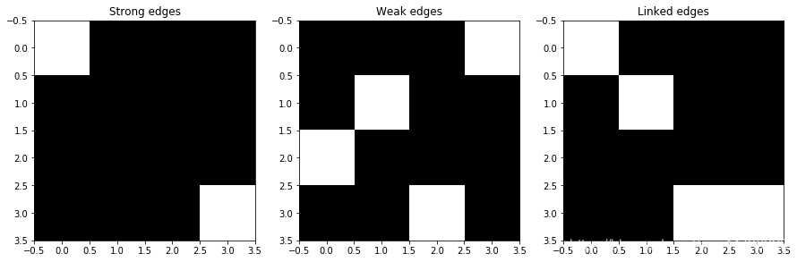
在上图中，白色方块代表存在边缘(包括强弱边缘)，遍历弱边缘中的每个像素，如果像素的八邻域存在强边缘对应的像素，则将这个弱边缘像素归为真正的边缘(从视觉上来理解，就是存在一条不确定的边缘，如果这条不确定的边缘旁存在真正的边缘，则将这条边归为真边，非则就将其删除)


可以看到相较于只保留弱边缘的效果图，滞后边界跟踪算法保留了更多的边缘细节。

整理一下整个算法，我们将Canny算子归纳到一个函数，调用一下看一下效果：

def canny(img, kernel_size=5, sigma=1.4, high=20, low=15):""" Implement canny edge detector by calling functions above.Args:img: binary image of shape (H, W).kernel_size: int of size for kernel matrix.sigma: float for calculating kernel.high: high threshold for strong edges.low: low threashold for weak edges.Returns:edge: numpy array of shape(H, W)."""### YOUR CODE HERE# 高斯模糊kernel = gaussian_kernel(kernel_size, sigma)img = conv(img, kernel)#io.imshow(color.gray2rgb(img))# 计算梯度Prewitt算子G, theta = gradient(img)#io.imshow(color.gray2rgb(G))# 非极大值抑制G = non_maximum_suppression(G, theta)#io.imshow(color.gray2rgb(G))# 双阈值抑制strong_edges, weak_edges = double_thresholding(G, high, low)# 连通边edge = link_edges(strong_edges, weak_edges)### END YOUR CODEreturn edge

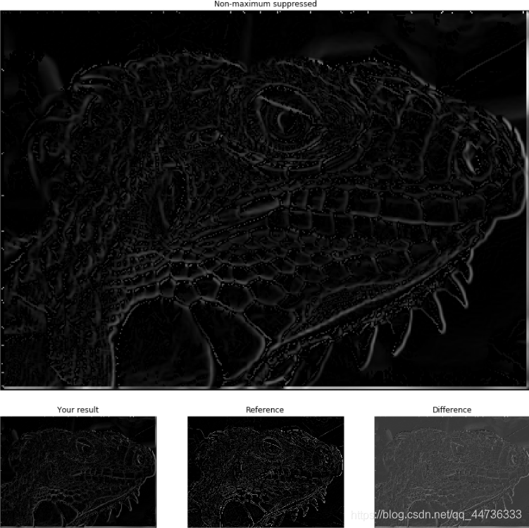
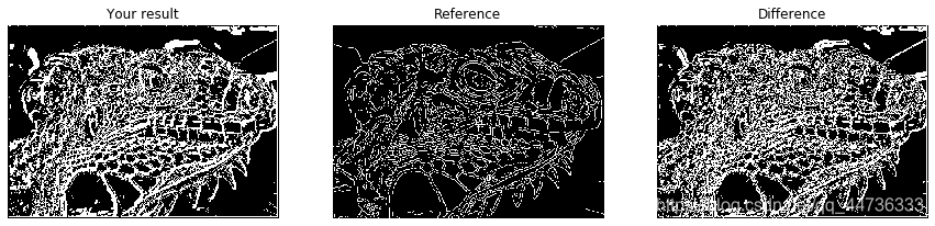
from edge import canny# Load image
img = io.imread('iguana.png', as_gray=True)# Run Canny edge detector
edges = canny(img, kernel_size=5, sigma=1.4, high=0.03, low=0.02)
print (edges.shape)plt.subplot(1, 3, 1)
plt.imshow(edges)
plt.axis('off')
plt.title('Your result')plt.subplot(1, 3, 2)
reference = np.load('references/iguana_canny.npy')
plt.imshow(reference)
plt.axis('off')
plt.title('Reference')plt.subplot(1, 3, 3)
plt.imshow(edges ^ reference)
plt.title('Difference')
plt.axis('off')
plt.show()

---

总结

这次写整个Canny算法其实遇到了很多坑，比如角度弧度换算那里，课件上写得很模糊，后来查阅资料才理清楚的。其次就是弱边界判断那里，我一开始对应每一个像素都要遍历整张图片的梯度方向，然后时间复杂度太大了，其实只要遍历八邻域就可以了。最后就是写代码一定要一定要细心，虽然python相较于c有很多东西都已经帮你写好了，但是还是要注意类似list下标之类的问题。
差不多就这样啦~