Linear Regression & Logistic Regression
Keywords List
keywords you may encounter when exploring LR(Logistic Regression), or a bigger concept – ML(machine learining):
监督学习 损失函数 梯度下降 学习率 激活函数 神经网络
Let’s kick off with Linear Regression
let’s dive into today’s topic in a data-oriented perspective·
So, we have massive data accumulated during last decades ,and it cannot help you with anything, doesnt make any sense at all, here comes the question, how do we make use of it?
Let’s start with a specific dataset, Boston housing, I believe we all have the experience to find ourselves a rented room in Beijing, it probably makes sense to you that if a place charges more, there gotta be something good with the place , what factors make people pay more? the NO.1 factor comes up to your mind might be this-- house area, but apparently it’s not rational enough that housing price depends on one single factor, well, in Boston housing dataset, there are 13 factors offered, let’s take a look at them:
EDA(Exploratory Data Analysis)- CRIM : 城镇人均犯罪率
- ZN : 住房用地超过 25000 平方尺的比例
- INDUS : 住房所在城镇非零售商用土地的比例
- CHAS : 有关查理斯河的虚拟变量(如果住房位于河边则为1,否则为0 )
- NOX : 一氧化氮浓度
- RM : 每栋住宅的房间数
- AGE : 1940 年以前建成的自住单位的比例
- DIS : 距离 5 个波士顿的就业中心的加权距离
- RAD : 距离高速公路的便利指数
- TAX : 每一万美元的不动产税率
- PTRATIO: 城镇中的教师学生比例
- B : 1000(Bk-0.63)^2,其中 Bk 指代城镇中黑人的比例
- LSTAT : 地区中有多少房东属于低收入人群
- MEDV : 自住房屋房价中位数(也就是均价)
boston = load_boston()
# print(boston.keys())
# # dict_keys(['data', 'target', 'feature_names', 'DESCR', 'filename'])
# dataframe加载数据
boston_df = pd.DataFrame(boston.data)
boston_df.columns = boston.feature_names
boston_df['PRICE'] = boston.target
print(boston_df.shape)
14 columns, the first 13 columns are independent variables here, MEDV the target, which we need to predict. Here comes our first concept : 监督学习(supervised learning)
监督学习(supervised learning) means samples come with targets or labels, while its antonym 非监督学习(unsupervised learning) means that all you have is independent variables .
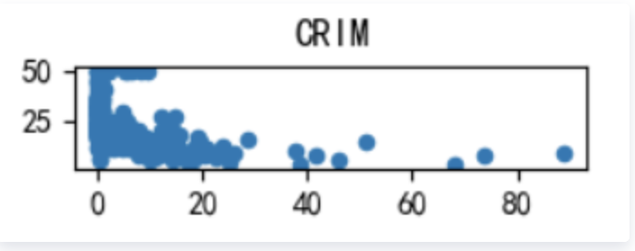
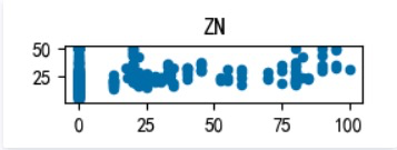
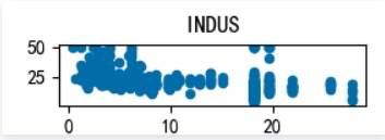
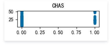
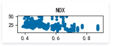
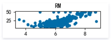
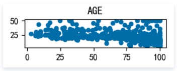
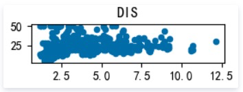
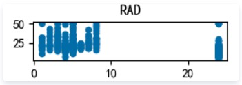
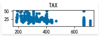
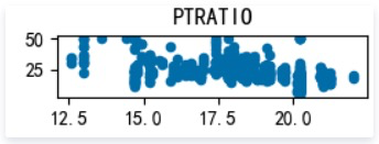
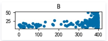
We’re gonna check the relationship between the target and the independent variable separately(Detailed in Boston_Housing.py), here are the scatter plots, let’s go through them:
CRIM: 城镇人均犯罪率
ZN: 住宅用地所占比例
INDUS: 城镇中非住宅用地所占比例
CHAS: 虚拟变量,用于回归分析
NOX: 环保指数
RM: 每栋住宅的房间数
AGE: 1940 年以前建成的自住单位的比例
DIS: 距离 5 个波士顿的就业中心的加权距离
RAD: 距离高速公路的便利指数
TAX: 每一万美元的不动产税率
PTRATIO: 城镇中的教师学生比例
B: 城镇中的黑人比例
LSTAT: 地区中有多少房东属于低收入人群
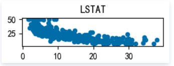
as we can see, MEDV varies linearly with 3 factors : RM(每栋住宅的房间数),LSTAT(地区中有多少房东属于低收入人群),PTRATIO(城镇中的教师学生比例), not every 13 factors, it’s still worth a try building a linear regression model to fit this dataset.
13 factors mean 13 independent variables in a function , 13 independent variables are plenty enough to build up a kingdom in hyperspace, but we are all trapped in 3D world, that’s totally beyond our imagination.
To ease you in, I’m gonna make another simple demo to illustrate, and we gonna learn another 3 keywords mentioned above in this demo –
损失函数(Loss Function), 梯度下降(gradient descend), 学习率(Learning Rate)
These keywords might be confusing for beginners, I hope you can crack them one by one during this demo, let’s check it out.
Simulation Data
# @Project :LR
# @Python :
# @Author : nivinanull@163.com
# @File : Linear_simulation.pyimport torch
import matplotlib.pyplot as plt
import sys
# 保证每次参数初始化都相同
torch.manual_seed(10)# 创建训练数据
# rand 包含了从区间[0, 1)的均匀分布中抽取的一组随机数
x = torch.rand(20, 1) * 10  # x data (tensor), shape=(20, 1)
# randn 包含了从标准正态分布(均值为0,方差为1,即高斯白噪声)中抽取的一组随机数
# y = 2x + 5 添加白噪声
y = 2*x + (5 + torch.randn(20, 1))  # y data (tensor), shape=(20, 1)# 首先描绘出散点,提出问题,怎样确定y = wx+b中 w和b的值
# 展示iteration循环迭代效果图
plt.scatter(x.data.numpy(), y.data.numpy())
plt.show()
# sys.exit()
First, we initiate x, then y, which is designed to vary roughly linearly with x. I hope the graph below can help you to catch the idea:
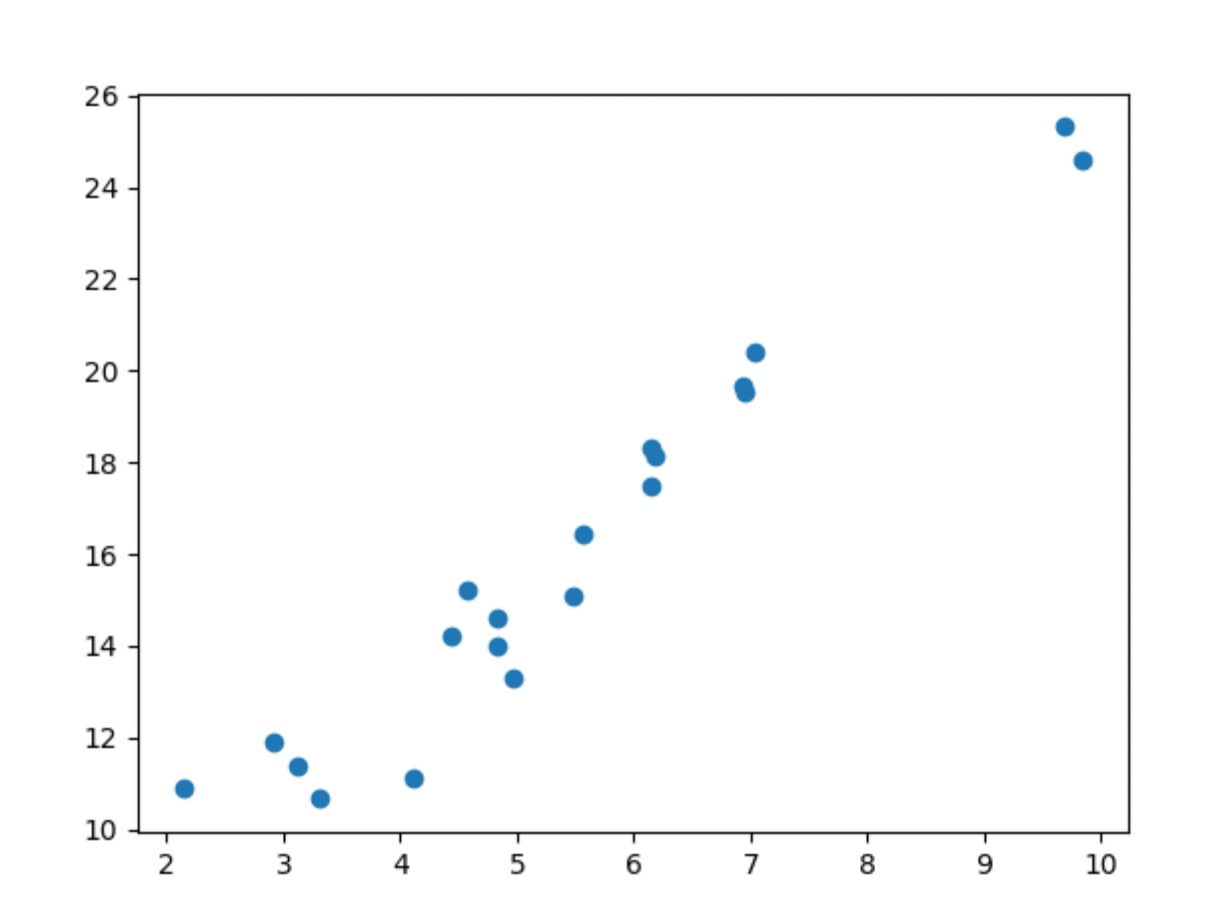
Here is the precondition, we know all the dots’ positions in the graph above, we list four of them:
(0, 5.5), (0.5, 5.8), (1, 7.72), (1.5, 8.3)
I believe anyone here can feel the linear relationship between x, y, but we are not able to write the equation down, let’s turn to computer for help.
(Run the linear_simulation.py)
(Run the linear_simulation.py)
(Run the linear_simulation.py)
大家请注意看参数 斜率w和截距b的变化!!!!!!!!!!!!!!!
大家请注意看参数 斜率w和截距b的变化!!!!!!!!!!!!!!!
大家请注意看参数 斜率w和截距b的变化!!!!!!!!!!!!!!!
(dont know how to make a gif…)
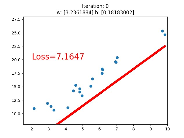
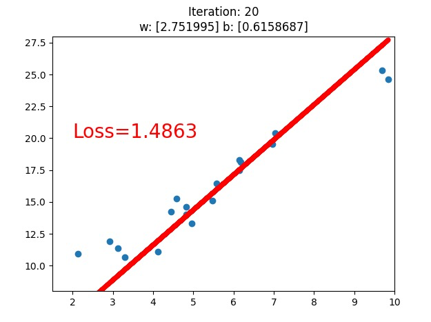
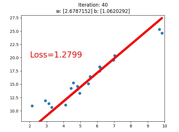
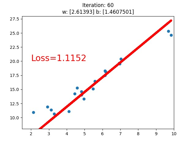
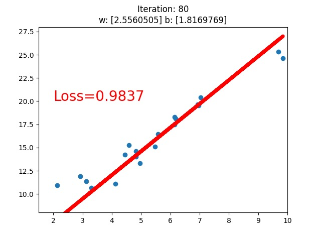
What does the computer do to solve the problem ? we tried two different conditions, loss.data.numpy() < 1, and loss.data.numpy() < 0.5(we only see the first version above), what we see is that the line fits better with this dataset, while what the computer know is that the loss value is going down.
The loss value , obviously, is the value of the loss function(损失函数), and we use gradient descend(梯度下降) to minimize the loss function, they work collaboratively on this job.
# 开始具体介绍以上概念
# 损失函数 确立靶心
# 梯度下降 数据指路
# 学习率调整 快走慢走lr = 0.05  # 学习率
for iteration in range(1000):# 前向传播wx = torch.mul(w, x)y_pred = torch.add(wx, b)# 计算 MSE lossloss = (0.5 * (y - y_pred) ** 2).mean()# 反向传播loss.backward()# 更新参数b.data.sub_(lr * b.grad)w.data.sub_(lr * w.grad)# 清零张量的梯度w.grad.zero_()b.grad.zero_()# 绘图if iteration % 20 == 0:plt.scatter(x.data.numpy(), y.data.numpy())# 颜色,线宽plt.plot(x.data.numpy(), y_pred.data.numpy(), 'r-', lw=5)plt.text(2, 20, 'Loss=%.4f' % loss.data.numpy(), fontdict={'size': 20, 'color':  'red'})plt.xlim(1.5, 10)plt.ylim(8, 28)plt.title("Iteration: {}\nw: {} b: {}".format(iteration, w.data.numpy(), b.data.numpy()))plt.pause(3)# 取loss.data.numpy() < 1 一次# 取loss.data.numpy() < 0.5 一次if loss.data.numpy() < 0.5:break
y^ is a denotation for predicted y(y^代表预测值)
y^ is a denotation for predicted y(y^代表预测值)
y^ is a denotation for predicted y(y^代表预测值)
Another question, how do we define the loss function(损失函数) ? In this case, we dont know the value of w and b at first, what we only know is that with an input x you get an predicted y^ (y^ = wx + b) and a real y, the target. and we want y^ approaches y as close as possible, how do we measure the difference between y^ and y?
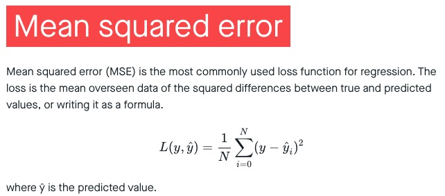
https://peltarion.com/knowledge-center/documentation/modeling-view/build-an-ai-model/loss-functions/mean-squared-error
I hope the picture above can ring a bell in your head, now we’re done with the Loss function part. Let’s move on to the next item – gradient descend(梯度下降) – a useful math tool to minimize the loss function
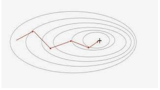
You may not be familiar with gradient (梯度), it’s about functions of several variables and their partial derivatives, and the concept of derivative might be a blur either, I recommend you to make an analogy between derivative and velocity which means the rate-of-change of position( If a function gives the position of something as a function of time, the first derivative gives its velocity, and the second derivative gives its acceleration), or the speed of sth in a particular direction , while the gradient represents the slope of the tangent of the graph of the function, more precisely, the gradient points in the direction of the greatest rate of increase of the function and its magnitude is the slope of the graph in that direction, so if we want to minimize the loss function, we take the opposite direction of gradient.

we got the loss function MSE above, we repalce y^ with ( wx + b):
L ( y , y ^ ) = 1 N ∑ i = 0 N ( y i − ( w x i + b ) ) 2 L(y, \hat y) = \frac {1}{N}\sum_{i=0}^{N}(y_i-(wx_i+b))^2 L(y,y^)=N1i=0∑N(yi−(wxi+b))2
then we take partial derivatives of w and b respectively:
− Δ w = − 1 N ∑ i = 0 N 2 x i ( y ^ i − y i ) -\Delta w = - \cfrac{1}{N}\sum_{i=0}^{N}2x_i(\hat y_i - y_i) −Δw=−N1i=0∑N2xi(y^i−yi)
− Δ b = − 1 N ∑ i = 0 N 2 ( y ^ i − y i ) -\Delta b = - \cfrac{1}{N}\sum_{i=0}^{N}2(\hat y_i - y_i) −Δb=−N1i=0∑N2(y^i−yi)
(These equations above are not the key point of our class, they are totally math thing, if you can’t trust them, try to prove them after)
For the forward propagation,we only get a predicted y^ equation with parameters w and b, it’s not a real number, and y^ is supposed to approach y as close as possible , then we found a way to measure the loss between y and y^, for the backward propagation, our target is clear,–minimizing the loss function, and we already found a math tool to fill the job, seems like we are all good to go, but how do we start ? we kind of got stuck in a delima here, y^ is an equation with parameters w and b, and w and b are supposed to vary in a way to minimize the loss function, but, as we can see here, y^ appeared in the derivative equations, the forward propagation and the backward propagation rely on each other like a vicious circle.
What do we do to break the vicious circle? we initiate the parameters randomly.
# 随机初始化线性回归参数w, b
w = torch.randn((1), requires_grad=True)
b = torch.zeros((1), requires_grad=True)
now we can update w and b with Δ w and Δb:
w = w + l r ( − Δ w ) w = w + lr(-\Delta w) w=w+lr(−Δw)
b = b + l r ( − Δ b ) b = b + lr(-\Delta b) b=b+lr(−Δb)
you might notice an unfamiliar symbol ‘lr’, what does that mean?,well, that’s our 4th keyword – learning rate(学习率), learning rate(学习率) means you dont update the parameters one hundred percent at a time with one single batch of data, it determines how large the update or moving step is, there definely will be misleadings in one batch of data, what learning rate(学习率) does is taking one small step a time towards the direction currently, it’s usually a small positive float less than 1 for the same reason. the value of the loss function will usually goes down with many many rounds of iterations. It’s a very important parameter. If lr is too small, then the algorithm might converge very slowly.
That reminds me of the story of how the world-known architect Walter Gropius got inspired by an aged lady selling grapes and designed the optimal paths for Disneyland , he suggested to have the seeds scattered all over the place at first, and here we initiate the parameters randomly, visitors are allowed to walk through the lawn until the track of paths is fixed, the idea behind it is to find paths that satisfies the most of the visitors, quite a tough job, as tough as the parameters need to fit most of the data (we dont take overfitting into account here),what we did is minimizing the loss function by moving towards the gradients using batches of data, what he did is following the paths that the lots of visitors trod, lots of visitors chose, people dont adapt their directions every single step though, it’s not a perfect analogy, I still bring it up just hoping you can gain more intuition between direction and gradient.I think it’s time to go back to the Boston housing example, I have some data processing tricks to show you.
(detaied in Boston_Housing.py)
if we still got plenty of time
So, we are all clear about what linear regression does and how the whole thing makes sense, how do we find a way to let the data talk in a classification task. I will make a start to logistic regression(there is a regression in it, but it’s used in classification tasks)
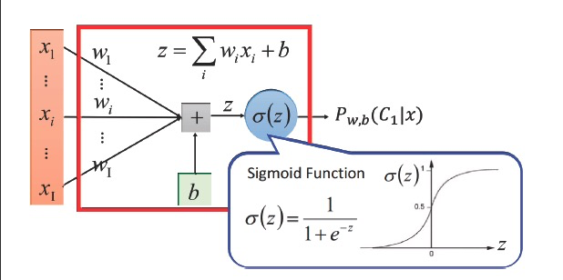
The activation function will do the trick for us, I’ll take the sigmoid activation function for example

The first glance at the formula gives us the information that with any real number as an input the function gives back a positive float between 0 and 1, just as the range of probability, so why not we see every output y as a probability of belonging to a classification category.
and the same way with linear regression, we set the loss function first, here is the most used loss function for logistic regression:Cross-Entropy Loss

https://blog.csdn.net/yinyu19950811/article/details/81321944
and you might still be confusing with the term activation function, I’d say the key point in it is “nonlinear”, during the linear regression part , you’ve seen that the only two operations used inside the prediction equation were the dot product and a sum. Both are linear operations.
If you add more layers but keep using only linear operations, then adding more layers would have no effect because each layer will always have some correlation with the input of the previous layer. This implies that, for a network with multiple layers, there would always be a network with fewer layers that predicts the same results.
What you want is to find an operation that makes the middle layers sometimes correlate with an input and sometimes not correlate.
You can achieve this behavior by using nonlinear functions. These nonlinear functions are called activation functions.
The single unit activated with a activation function in logistic regression is a basic neuron in neural network, it consists a neural network as a hidden unit。
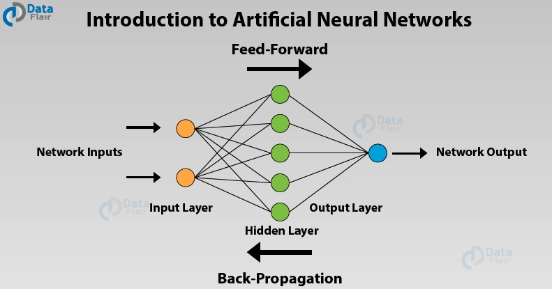
what does neural network, or deep learning have to do with the brain? At the risk of giving away the punchline, I would say not a whole lot. But let’s take a quick look at why people keep making the analogy between deep learning and the human brain. When you implement a neural network, this is what you do, forward prop and back prop. I think because it’s been difficult to convey intuitions about what these equations are doing really gradient descent on a very complex function, the analogy that is like the brain has become really an oversimplified explanation for what this is doing, but the simplicity of this makes it seductive for people to just say it publicly, as well as, for media to report it, and certainly caught the popular imagination. There is a very loose analogy between, let’s say a logistic regression unit with a sigmoid activation function, and here’s a cartoon of a single neuron in the brain.
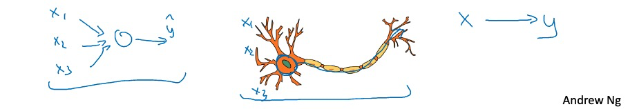
In this picture of a biological neuron, this neuron, which is a cell in your brain, receives electric signals from your other neurons, X_1, X_2, X_3, or maybe from other neurons A_1, A_2, A_3, does a simple thresholding computation, and then if this neuron fires, it sends a pulse of electricity down the axon, down this long wire perhaps to other neurons. So, there is a very simplistic analogy between a single neuron in a neural network and a biological neuron-like that shown on the right, but I think that today even neuroscientists have almost no idea what even a single neuron is doing. A single neuron appears to be much more complex than we are able to characterize with neuroscience, and while some of what is doing is a little bit like logistic regression, there’s still a lot about what even a single neuron does that no human today understands. For example, exactly how neurons in the human brain learns, is still a very mysterious process. It’s completely unclear today whether the human brain uses an algorithm, does anything like back propagation or gradient descent or if there’s some fundamentally different learning principle that the human brain uses? So, when I think of deep learning, I think of it as being very good at learning very flexible functions, very complex functions to learn X to Y mappings, to learn input-output mappings in supervised learning. Whereas this is like the brain analogy, maybe that was useful ones. I think the field has moved to the point where that analogy is breaking down and I tend not to use that analogy much anymore. So, that’s it for neural networks and the brain. I do think that maybe the few that computer vision has taken a bit more inspiration from the human brain than other disciplines that also apply deep learning, but I personally use the analogy to the human brain less than I used to
The following pictures are from a research of what layers of neuros do in a CV(Computer Vision) neural network, I hope you are able to gain more intuition about neural network.


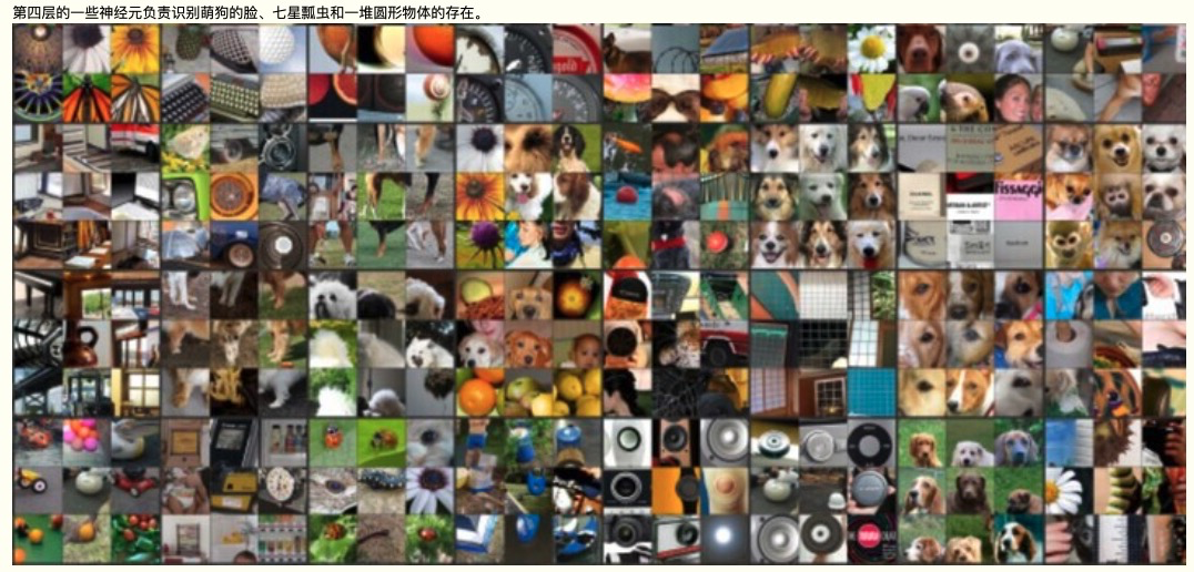
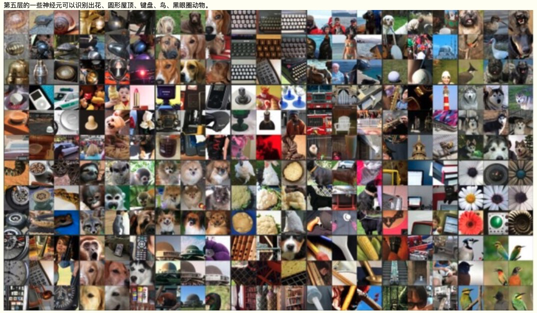
https://www.cnblogs.com/peizhe123/p/4641149.html?from=liebao_fast&did=oxuw4omg2vsj8muu5oc7boljkkq2
I guess this is it, and I hope u had a great time with me, Thank You!!!


![[JAVA实现]微信公众号网页授权登录,java开发面试笔试题](https://images.cnblogs.com/OutliningIndicators/ExpandedBlockStart.gif)