CVPR-2016
在 CIFAR-10 上的小实验可以参考博客【Keras-Inception v3】CIFAR-10

---

---

1 Background and Motivation

Although increased model size and computational cost tend to translate to immediate quality gains for most tasks (as long as enough labeled data is provided for training), computational efficiency and low parameter count are still enabling factors for various use cases such as mobile vision and big-data scenarios.

本文对GoogleNet 做了改进，目的是为了 computational efficiency

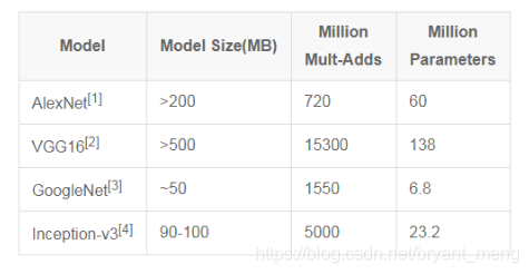
几种经典模型的尺寸，计算量和参数数量对比 ¹

2 Advantages / Contributions

describing a few general principles and optimization ideas to scale up convolution networks in efficient ways

design principles 是推测性（speculative）的，有待进一步的实验验证，但是如果严重偏离这些 principles 的话，效果会不好。所以设计网络的时候，见不贤而内自省也

design principles 具体如下

• Avoid representational bottlenecks, especially early in the network. 即feature map的大小不应该出现急剧的衰减，信息过度的压缩，将会丢失大量的信息，对模型的训练也造成了困难。
  理论上 information content can not be assessed merely by the dimensionality of the representation（h×w×c），因为丢失了一些重要信息，例如 correlation structure。维度只能 rough estimate of information content.

• Higher dimensional representations are easier to process locally within a network.
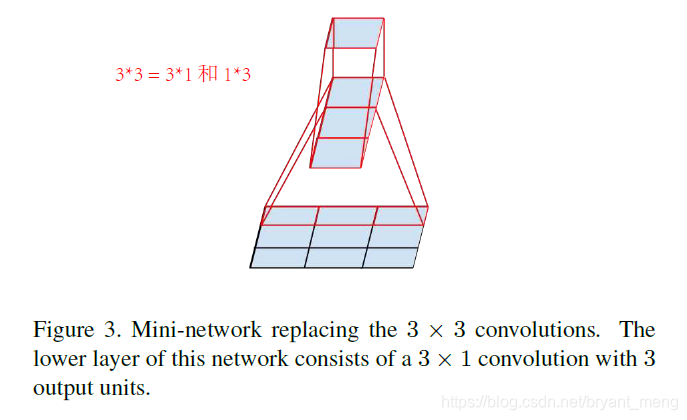
  在网络中对高维的表达进行局部的处理，将会使网络的训练增快。（3×3 = 1×3 + 3×1）

• Spatial aggregation can be done over lower dimensional embeddings without much or any loss in representational power. 因为feature map上，临近区域上的表达具有很高的相关性，如果对输出进行空间聚合，那么将feature map的维度降低也不会减少表达的信息。这样的话，有利于信息的压缩，并加快了训练的速度。（5×5 = 两个 3×3）

• Balance the width and depth of the network，要使得计算资源平衡的分配在模型的深度和宽度上面，才能最大化的提高模型的性能

3 Innovations

• suitably factorized convolutions，5×5 = 两个 3×3，3×3 = 1×3 + 3×1
• aggressive regularization，Label Smoothing

4 Method

• suitably factorized convolutions
• aggressive regularization

4.1 Factorizing Convolutions with Large Filter Size

4.1.1 Factorization into smaller convolutions

5×5 = 两个3×3

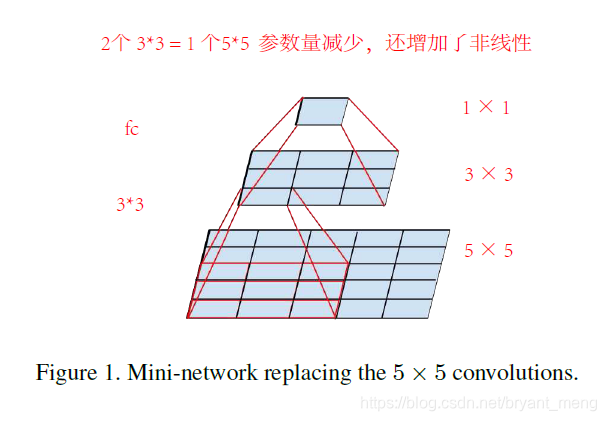
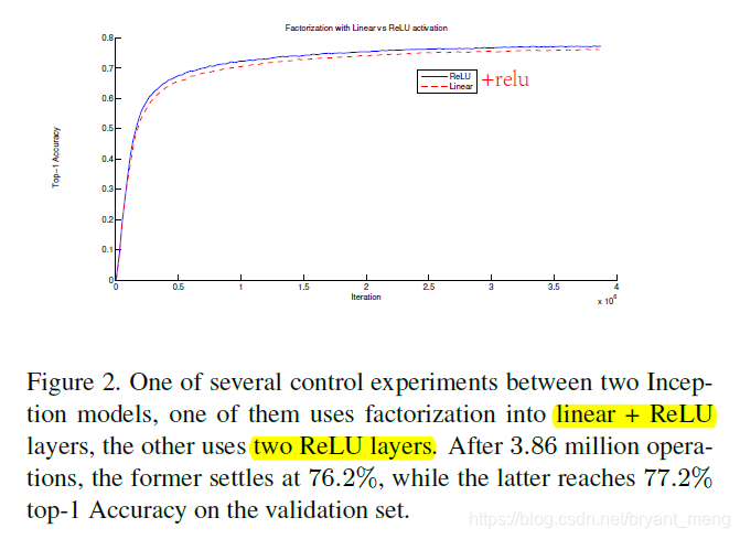
双 Relu vs linear + Relu ，前者胜

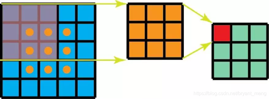
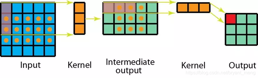
4.1.2 Spatial Factorization into Asymmetric Convolutions

能继续缩小吗？比如 3×3 = 2 个 2×2，可以。作者提出用 1×3+3×1，牛……

$\frac{3\times 3-2\times 2\times 2}{3\times 3}=11\%$

$\frac{3\times 3-(1\times 3+3\times 1)}{3\times 3}=33\%$

升华下 n×n 压缩成 1×n + n×1，实验表明，grid-sizes 在12-20之间的时候用这种方法压缩比较有用，n用7

4.2 Utility of Auxiliary Classifiers

有趣的是，实验表明 Auxiliary Classifiers 并不能加速 converge，只是在训练快要结束的时候，the network with the auxiliary branches starts to overtake the accuracy of the network without any auxiliary.

更详细的讨论见 【Inception v1】《Going Deeper with Convolutions》 的 第8节GoogleNet

4.3 Efficient Grid Size Reduction

Grid Size 指的是 feature map 的 size（不算 channels），也即 W 和 H
我们要把 $d\times d\times k\to \frac{d}{2}\times \frac{d}{2}\times 2k$

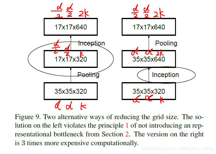
图中左边的结构先 pooling 再 convolution，operation（集中在 convolution）为 $\frac{d}{2}\times \frac{d}{2}\times k\times 2k$

图中右边的结构先 convolution 再 pooling，operation（集中在 convolution）为 $d\times d\times k\times 2k$

Notice：operation 和 parameters 的区别，parameters 的计算只与 filter size 和 feature maps 的 channels 有关，与 feature maps 的 size 无关

虽然图中左边的结构 operation 少很多，但是 违背 principle 1（Avoid representational bottlenecks, especially early in the network）

作者的做法如下

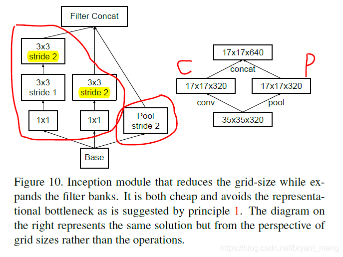
这样做就避免了违背 principle 1

4.4 Inception-v3

caffe代码 + caffe代码可视化工具

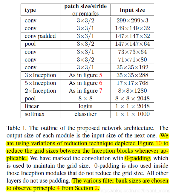
reduction technique 见本博客4.3节图 10，表中的 inception 细节如下面图所示

把传统的第一步 7×7 变成了 3个 3×3

---

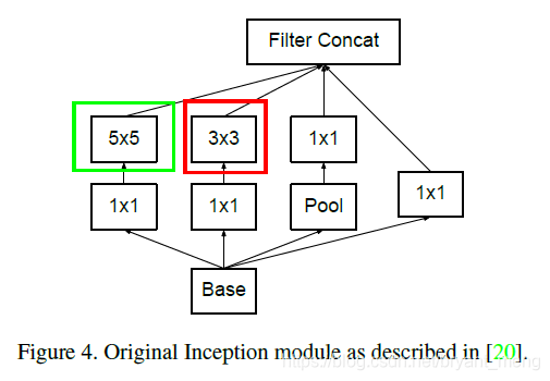
• Inception-v1（原版）

---

重复3次

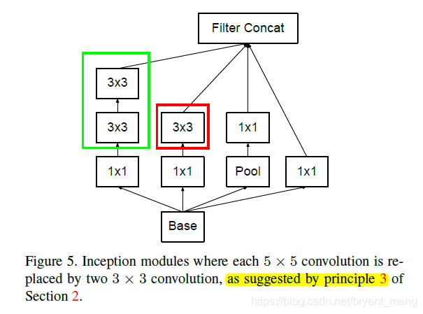
principle 3：Spatial aggregation can be done over lower dimensional embeddings without much or any loss in representational power.

---

重复5次

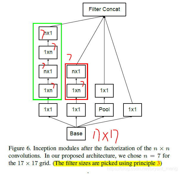
Principle 3：Spatial aggregation can be done over lower dimensional embeddings without much or any loss in representational power.

---

重复2次

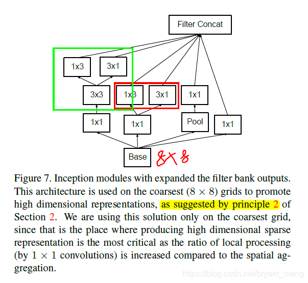
Principle 2：Higher dimensional representations are easier to process locally within a network.

---

4.5 Model Regularization via Label Smoothing

• label：$k\in ｛1...K｝$
• softmax：$p(k|x)=\frac{exp(z_k)}{{\sum }_{i=1}^{K}exp(z_i)}$，其中 $z_i=w\ast x+b$
• ground-truth distribution：$q(k|x)$，且 ${\sum }_{k}q(k|x)=1$，因为只有一类为1，其它都为0
• cross-entropy loss：$l={\sum }_{k=1}^{K}q(k)\cdot log(p(k))$
• gradient：$\frac{\partial l}{\partial z_k}=p(k)-q(k)$，参考 简单易懂的softmax交叉熵损失函数求导

假设某个样本的 label 为$y$，作者发现，最小化 loss 等于最大化 $logp(k)$，这样会导致 $z_y\gg z_k$，softmax 公式中可以看出 $exp(z_k)$ 是活力无限的（no limit）。logit corresponding to the ground-truth label is much great than all other logits. 这样会导致两个问题

• result in over-fitting
• reduces the ability of the model to adapt

Intuitively, this happens because the model becomes too confident about its predictions. 也可以理解为平时模拟的时候把某种题型做的太多了，太膨胀（得瑟）了！

为了那我们的model别那么得瑟（overfitting），作者提出了改进
上述的 $q(k)={\delta }_{k,y}$，${\delta }_{k,y}$ is Dirac delta（ 狄拉克δ函数(Dirac delta)和狄拉克梳状函数(Dirac comb)）

$q(k)=\{\begin{array}{cc}1& k=y\\ 0& k\ne y\end{array}$

改进，加入了一个 $u(k)$ distribution（论文中是 uniform distribution） 和 smoothing parameter $ϵ=0.1$

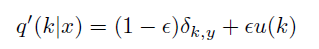
$u(k)=\frac{1}{K}$，independent of the training example，with probability $ϵ$, replace k with a sample drawn from the distribution u(k).

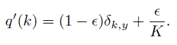
感觉改进是这样子的，把 0，1标签改得 soft target 一些（鄙人拙见），文中直观的说法是 all q′(k) have a positive lower bound.

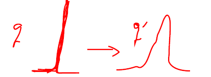
作者把他叫做 label-smoothing regularization, or LSR.

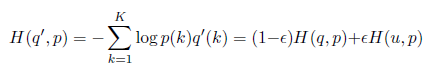
LSR is equivalent to replacing a single cross-entropy loss $H(q,p)$ with a pair of such losses $H(q,p)$ and $H(u,p)$.

进一步化简（参考 详解机器学习中的熵、条件熵、相对熵和交叉熵）

• $H(u,p)=-u\cdot logp=u\cdot log\frac{1}{p}$，cross entropy——可以来衡量在给定的真实分布下，使用非真实分布所指定的策略消除系统的不确定性所需要付出的努力的大小
• $H(u)=-u\cdot logu=u\cdot log\frac{1}{u}$：信息熵
• $D_{KL}(u||p)=u\cdot log\frac{u}{p}$：相对熵（也叫 KL divergence）——可以用来衡量两个概率分布之间的差异。

从上面公式可以看出，$H(u,p)=H(u)+D_{KL}(u||p)$

说明，作者改进版本添加的第二项就是$H(u,p)$ 指的是 p 和 u 概率分布之间的差距，让模型学习得雨露均沾一点，别那么一枝独秀（u 是 uniform 分布之后，$H(u)$ 是定值）

用 $-H(p)$ 也能起到和 $H(u,p)$ 相同的作用，p（softmax后的结果）越纯，$H(p)$ 越小，$-H(p)$越大，也惩罚了这种一枝独秀的情况。

---

label smoothing 的 pytorch 实现如下，参考 【Pytorch】label smoothing 和 label smoothing理论及PyTorch实现

import torch
import torch.nn as nnclass NMTCritierion(nn.Module):"""TODO:1. Add label smoothing"""def __init__(self, label_smoothing=0.0):super(NMTCritierion, self).__init__()self.label_smoothing = label_smoothingself.LogSoftmax = nn.LogSoftmax()if label_smoothing > 0:self.criterion = nn.KLDivLoss(size_average=False)else:self.criterion = nn.NLLLoss(size_average=False, ignore_index=100000)self.confidence = 1.0 - label_smoothingdef _smooth_label(self, num_tokens):# When label smoothing is turned on,# KL-divergence between q_{smoothed ground truth prob.}(w)# and p_{prob. computed by model}(w) is minimized.# If label smoothing value is set to zero, the loss# is equivalent to NLLLoss or CrossEntropyLoss.# All non-true labels are uniformly set to low-confidence.one_hot = torch.randn(1, num_tokens)one_hot.fill_(self.label_smoothing / (num_tokens - 1))return one_hotdef _bottle(self, v):return v.view(-1, v.size(2))def forward(self, dec_outs, labels):scores = self.LogSoftmax(dec_outs)num_tokens = scores.size(-1)# conduct label_smoothing modulegtruth = labels.view(-1)if self.confidence < 1:tdata = gtruth.detach()one_hot = self._smooth_label(num_tokens)  # Do label smoothing, shape is [M]if labels.is_cuda:one_hot = one_hot.cuda()tmp_ = one_hot.repeat(gtruth.size(0), 1)  # [N, M]tmp_.scatter_(1, tdata.unsqueeze(1), self.confidence)  # after tdata.unsqueeze(1) , tdata shape is [N,1]gtruth = tmp_.detach()loss = self.criterion(scores, gtruth)return loss

5 Dataset

ILSVRC-2012

6 Experiments

训练的时候用到了

• RMSProp
• gradient clipping with threshold 2.0

6.1 Performance on Lower Resolution Input

这里的实验我不是特别理解


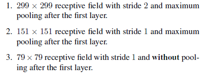
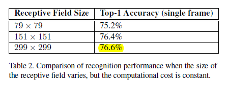
结论：one might consider using dedicated high-cost low resolution networks for smaller objects in the R-CNN [5] context.

6.2 Experimental Results and Comparisons

ILSVRC-2012 validation set

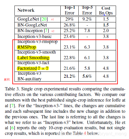
v3-basic 不晓得是什么样的版本，auxiliary 分类器中加 BN还是可以的。注意红色框框是累积的实验结果，也就是后面的实验也有前面的实验的东西。Factorized 7 × 7 includes a change that factorizes the first 7 × 7 convolutional layer into a sequence of 3 × 3 convolutional layers.

---

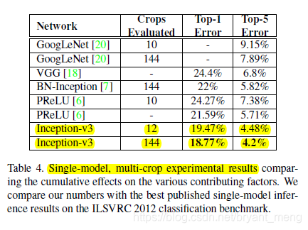
solo 王

---

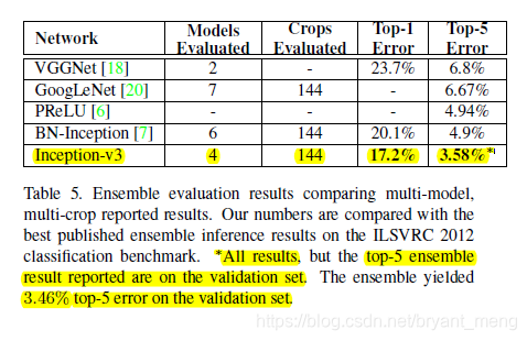
ensemble

7 Conclusion

several design proposal

ILSVRC-2012 上 state-of-art，2.5 × BN 计算量（v2）

• Q1：4 个design principle 的形象化理解，结合图 5，6，7
• Q2：softmax 中太过自信导致的两个问题的理解
• Q3：6.1 小节 Lower Resolution Input 中 receptive filed 指的是什么意思呢？
• Q4：关于 Auxiliary Classifiers 的思考，结合 【Inception-v1】《Going Deeper with Convolutions》 最后一小节 GoogleNet

附录（Spatial Factorization）

参考文章 一文读懂 12种卷积方法（含1x1卷积、转置卷积和深度可分离卷积等）

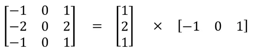
上面是 sobel 算子
1个 $3\ast 3$ 可以分解成一个 $1\ast 3$ 和 1个 $3\ast 1$

传统卷积计算量为：$3\ast 3\ast 3\ast 3=81（kernelsize\ast outputsize）$

Spatial Factorization 的计算量 $1\ast 3\ast 3\ast 5+3\ast 1\ast 3\ast 3=45+27=72（kernelsize\ast outputsize）$

泛化一下（kernel size 为 $k$，output size 为 $h\ast w$）：

• 正常卷积：$k\ast k\ast h\ast w$
• Spatial Factorization convolution：$k\ast 1\ast (h-k+1)\ast w+1\ast k\ast h\ast w$

如果 $h,w$ 远远大于 $k$，那么计算成本比为

$$\frac{2\ast k\ast h\ast w}{k\ast k\ast h\ast w}=\frac{2}{k}$$

缺点，尽管 Spatial Factorization convolution 能节省成本，但深度学习却很少使用它，主要原因是，并非所有的核都能分解成两个更小的核，如果用两个小核代替一个大核，会减少搜索所有可能的核，这样可能得到的结果不是最优的！

---

1. 五种CNN模型的尺寸，计算量和参数数量对比详解 ↩︎