目录
导包和处理数据
数据预处理--减平均值和把偏置并入权重
SVM
naive版
向量版
向量版
线性分类器--采用SGD算法
SVM版线性分类
Softmax版线性分类
使用验证集调试学习率和正则化系数
画出结果
测试准确率
可视化权重
值得注意的地方
赋值
randrange
np.arange
np.random.choice
np.random.permutation
random.shuffle
导包和处理数据
值得一提的是,这里在训练集中额外分出一个dev集,到最后也不知道有啥用
# Run some setup code for this notebook.
import random
import numpy as np
from cs231n.data_utils import load_CIFAR10
import matplotlib.pyplot as plt
import time# This is a bit of magic to make matplotlib figures appear inline in the
# notebook rather than in a new window.
%matplotlib inline
plt.rcParams['figure.figsize'] = (10.0, 8.0) # set default size of plots
plt.rcParams['image.interpolation'] = 'nearest'
plt.rcParams['image.cmap'] = 'gray'# Some more magic so that the notebook will reload external python modules;
# see http://stackoverflow.com/questions/1907993/autoreload-of-modules-in-ipython
%load_ext autoreload
%autoreload 2# Load the raw CIFAR-10 data.
cifar10_dir = 'cs231n\datasets\CIFAR10'# Cleaning up variables to prevent loading data multiple times (which may cause memory issue)
try:del X_train, y_traindel X_test, y_testprint('Clear previously loaded data.')
except:passX_train, y_train, X_test, y_test = load_CIFAR10(cifar10_dir)# As a sanity check, we print out the size of the training and test data.
print('Training data shape: ', X_train.shape)
print('Training labels shape: ', y_train.shape)
print('Test data shape: ', X_test.shape)
print('Test labels shape: ', y_test.shape)# Split the data into train, val, and test sets. In addition we will
# create a small development set as a subset of the training data;
# we can use this for development so our code runs faster.
num_training = 49000
num_validation = 1000
num_test = 1000
num_dev = 500# Our validation set will be num_validation points from the original
# training set.
mask = range(num_training, num_training + num_validation)
X_val = X_train[mask]
y_val = y_train[mask]# Our training set will be the first num_train points from the original
# training set.
mask = range(num_training)
X_train = X_train[mask]
y_train = y_train[mask]# We will also make a development set, which is a small subset of the training set.
mask = np.random.choice(num_training, num_dev, replace=False)
X_dev = X_train[mask]
y_dev = y_train[mask]# We use the first num_test points of the original test set as our test set.
mask = range(num_test)
X_test = X_test[mask]
y_test = y_test[mask]print('Train data shape: ', X_train.shape)
print('Train labels shape: ', y_train.shape)
print('Validation data shape: ', X_val.shape)
print('Validation labels shape: ', y_val.shape)
print('Test data shape: ', X_test.shape)
print('Test labels shape: ', y_test.shape)# Preprocessing: reshape the image data into rows
X_train = np.reshape(X_train, (X_train.shape[0], -1))
X_val = np.reshape(X_val, (X_val.shape[0], -1))
X_test = np.reshape(X_test, (X_test.shape[0], -1))
X_dev = np.reshape(X_dev, (X_dev.shape[0], -1))# As a sanity check, print out the shapes of the data
print('Training data shape: ', X_train.shape)
print('Validation data shape: ', X_val.shape)
print('Test data shape: ', X_test.shape)
print('dev data shape: ', X_dev.shape)
数据预处理--减平均值和把偏置并入权重
# Preprocessing: subtract the mean image
# first: compute the image mean based on the training data
mean_image = np.mean(X_train, axis=0)  # shape: (3072,)plt.figure(figsize=(4,4))
plt.imshow(mean_image.reshape((32,32,3)).astype('uint8')) # visualize the mean image
plt.show()# second: subtract the mean image from train and test data
X_train -= mean_image
X_val -= mean_image
X_test -= mean_image
X_dev -= mean_image# third: append the bias dimension of ones (i.e. bias trick) so that our SVM
# only has to worry about optimizing a single weight matrix W.
X_train = np.hstack([X_train, np.ones((X_train.shape[0], 1))])
X_val = np.hstack([X_val, np.ones((X_val.shape[0], 1))])
X_test = np.hstack([X_test, np.ones((X_test.shape[0], 1))])
X_dev = np.hstack([X_dev, np.ones((X_dev.shape[0], 1))])print(X_train.shape, X_val.shape, X_test.shape, X_dev.shape)
SVM
naive版
# linear_svm.pyimport numpy as np
from random import shuffledef svm_loss_naive(W, X, y, reg):"""Inputs:- W: A numpy array of shape (D, C) containing weights.- X: A numpy array of shape (N, D) containing a minibatch of data.- y: A numpy array of shape (N,) containing training labels; y[i] = c meansthat X[i] has label c, where 0 <= c < C.- reg: (float) regularization strengthReturns a tuple of:- loss as single float- gradient with respect to weights W; an array of same shape as W"""dW = np.zeros(W.shape)  # initialize the gradient as zero# compute the loss and the gradientnum_classes = W.shape[1]num_train = X.shape[0]loss = 0.0for i in range(num_train):scores = X[i].dot(W)correct_class_score = scores[y[i]]for j in range(num_classes):if j == y[i]:continuemargin = scores[j] - correct_class_score + 1  # note delta = 1if margin > 0:loss += margindW[:, j] += X[i]  # W的第j列是针对第j类的权重,对sj有贡献dW[:, y[i]] -= X[i] # dW[:, j]和X[i]形状都是(3073,),所以可以赋值loss /= num_trainloss += reg * np.sum(W * W)dW /= num_traindW += 2 * W * regreturn loss, dW
向量版
def svm_loss_vectorized(W, X, y, reg):"""Structured SVM loss function, vectorized implementation."""loss = 0.0dW = np.zeros(W.shape) # initialize the gradient as zeroscores = X.dot(W) # N, Cnum_class = W.shape[1]num_train = X.shape[0]correct_class_score = scores[np.arange(num_train), y] # shape: (num_class,) correct_class_score = correct_class_score.reshape([-1, 1]) # shape: (num_class,1) loss_tep = scores - correct_class_score + 1loss_tep[loss_tep < 0] = 0 # 求与0相比的最大值# loss_tep = np.maximum(0, loss_tep)loss_tep[np.arange(num_train), y] = 0 # 正确的类loss为0loss = loss_tep.sum()/num_train + reg * np.sum(W * W)# loss_tep等于0的位置,对X的导数就是0# loss_tep元素大于0的位置,说明此处有loss,对于非正确标签类的S求导为1loss_tep[loss_tep > 0] = 1 # N, C # 对于正确标签类,每有一个loss_tep元素大于0,则正确标签类的S求导为-1,要累加loss_item_count = np.sum(loss_tep, axis=1) loss_tep[np.arange(num_train), y] -= loss_item_count #在一次错误的分类中,# dW中第i,j元素对应于第i维,第j类的权重# X.T的第i行每个元素对应于每个样本第i维的输入,正是Sj对W[i,j]的导数# loss_tep的第j列每个元素对应于每个样本在第j类的得分是否出现,相当于掩码# X.T和loss_tep的矩阵乘法等于对每个样本的W[i,j]导数值求和# 简单地说,就是loss对S的导数是loss_tep, loss_tep对W的导数是X.TdW = X.T.dot(loss_tep) / num_train # (D, N) *(N, C) dW += 2 * reg * Wreturn loss, dWSoftmax
navie版
def softmax_loss_naive(W, X, y, reg):"""Inputs:- W: A numpy array of shape (D, C) containing weights.- X: A numpy array of shape (N, D) containing a minibatch of data.- y: A numpy array of shape (N,) containing training labels; y[i] = c meansthat X[i] has label c, where 0 <= c < C.- reg: (float) regularization strengthReturns a tuple of:- loss as single float- gradient with respect to weights W; an array of same shape as W"""# Initialize the loss and gradient to zero.loss = 0.0dW = np.zeros_like(W)num_train = X.shape[0]num_class = W.shape[1]for i in range(num_train):scores = X[i].dot(W)f = scores - np.max(scores) # 防止指数过大,计算溢出softmax = np.exp(f) / np.exp(f).sum() loss += -np.log(softmax[y[i]]) # log()是自然底数dW[:, y[i]] += -X[i] # y[i]和其他项相比多了-fyi这一项,for j in range(num_class):dW[:, j] += X[i] * softmax[j] # ln(∑e^fi)对W[i,j]求导loss /= num_traindW /= num_trainloss += reg * np.sum(W ** 2)dW += 2 * reg * Wreturn loss, dW测试,初始计算的loss应该是-log(0.1)
# First implement the naive softmax loss function with nested loops.
# Generate a random softmax weight matrix and use it to compute the loss.
W = np.random.randn(3073, 10) * 0.0001
loss, grad = softmax_loss_naive(W, X_dev, y_dev, 0.0)# As a rough sanity check, our loss should be something close to -log(0.1).
print('loss: %f' % loss)
print('sanity check: %f' % (-np.log(0.1)))
loss: 2.367920 sanity check: 2.302585
向量版
def softmax_loss_vectorized(W, X, y, reg):"""Softmax loss function, vectorized version.Inputs and outputs are the same as softmax_loss_naive."""# Initialize the loss and gradient to zero.loss = 0.0dW = np.zeros_like(W)num_trains = X.shape[0]num_calss = W.shape[1]scores = X.dot(W) # (N, C)max_val = np.max(scores, axis=1).reshape(-1, 1) # 求每一个样本中的最大得分f = scores - max_val # 防止指数过大,计算溢出softmax = np.exp(f)/ np.exp(f).sum(axis=1).reshape(-1,1)loss_i = -np.log(softmax[np.arange(num_trains), y]).sum() # 将分类正确的softmax取出loss += loss_isoftmax[np.arange(num_trains), y] -= 1 #处理log的分子项的导数dW = X.T.dot(softmax) # dW[:, j] += X[i] * softmax[j]的向量化loss /= num_trainsdW /= num_trainsloss += reg * np.sum(W * W)dW += 2 * reg * W# *****END OF YOUR CODE (DO NOT DELETE/MODIFY THIS LINE)*****return loss, dW
线性分类器--采用SGD算法
巧妙的地方是定义了一个模板,loss让子类来实现,这样可以使用不同的loss函数
# inear_classifier.py.class LinearClassifier(object):def __init__(self):self.W = Nonedef train(self,X,y,learning_rate=1e-3,reg=1e-5,num_iters=100,batch_size=200,verbose=False,):"""Train this linear classifier using stochastic gradient descent.Inputs:- X: A numpy array of shape (N, D) containing training data; there are Ntraining samples each of dimension D.- y: A numpy array of shape (N,) containing training labels; y[i] = cmeans that X[i] has label 0 <= c < C for C classes.- learning_rate: (float) learning rate for optimization.- reg: (float) regularization strength.- num_iters: (integer) number of steps to take when optimizing- batch_size: (integer) number of training examples to use at each step.- verbose: (boolean) If true, print progress during optimization.Outputs:A list containing the value of the loss function at each training iteration."""num_train, dim = X.shapenum_classes = (np.max(y) + 1) # assume y takes values 0...K-1 where K is number of classesif self.W is None:# lazily initialize Wself.W = 0.001 * np.random.randn(dim, num_classes)# Run stochastic gradient descent to optimize Wloss_history = []for it in range(num_iters):X_batch = Noney_batch = Nonemask = np.random.choice(num_train, batch_size, replace=True)# replace=True代表选出来的样本可以重复。# 每次迭代都是重新随机选样本组成batch,意味着有些会选不到,有点会被重复选。有些粗糙X_batch = X[mask]y_batch = y[mask]# evaluate loss and gradientloss, grad = self.loss(X_batch, y_batch, reg)loss_history.append(loss)self.W -= learning_rate * gradif verbose and it % 100 == 0:print("iteration %d / %d: loss %f" % (it, num_iters, loss))return loss_historydef predict(self, X):"""Use the trained weights of this linear classifier to predict labels fordata points.Inputs:- X: A numpy array of shape (N, D) containing training data; there are Ntraining samples each of dimension D.Returns:- y_pred: Predicted labels for the data in X. y_pred is a 1-dimensionalarray of length N, and each element is an integer giving the predictedclass."""y_pred = np.zeros(X.shape[0])y_pred = np.argmax(X.dot(self.W), axis = 1) # (N, D) * (D, C)return y_preddef loss(self, X_batch, y_batch, reg):"""Compute the loss function and its derivative.Subclasses will override this."""passSVM版线性分类
class LinearSVM(LinearClassifier):""" A subclass that uses the Multiclass SVM loss function """def loss(self, X_batch, y_batch, reg):return svm_loss_vectorized(self.W, X_batch, y_batch, reg)训练
svm = LinearSVM()
tic = time.time()
loss_hist = svm.train(X_train, y_train, learning_rate=1e-7, reg=2.5e4,num_iters=1500, verbose=True)
toc = time.time()
print('That took %fs' % (toc - tic))
# Write the LinearSVM.predict function and evaluate the performance on both the
# training and validation set
y_train_pred = svm.predict(X_train)
print('training accuracy: %f' % (np.mean(y_train == y_train_pred), ))
y_val_pred = svm.predict(X_val)
print('validation accuracy: %f' % (np.mean(y_val == y_val_pred), ))
Softmax版线性分类
class Softmax(LinearClassifier):""" A subclass that uses the Softmax + Cross-entropy loss function """def loss(self, X_batch, y_batch, reg):return softmax_loss_vectorized(self.W, X_batch, y_batch, reg)使用验证集调试学习率和正则化系数
# Note: you may see runtime/overflow warnings during hyper-parameter search.
# This may be caused by extreme values, and is not a bug.
results = {}
best_val = -1   # The highest validation accuracy that we have seen so far.
best_svm = None # The LinearSVM object that achieved the highest validation rate.################################################################################
# Hint: You should use a small value for num_iters as you develop your         #
# validation code so that the SVMs don't take much time to train; once you are #
# confident that your validation code works, you should rerun the validation   #
# code with a larger value for num_iters.                                      #
################################################################################# Provided as a reference. You may or may not want to change these hyperparameters
learning_rates = [1e-7, 1e-6]
regularization_strengths = [2.5e4, 5e4]for rate in learning_rates:for strength in regularization_strengths:svm = LinearSVM()svm.train(X_train, y_train, learning_rate=rate, reg=strength,num_iters=1500, verbose=True)y_train_pred = svm.predict(X_train,)training_accuracy = np.mean(y_train_pred == y_train)y_val_pred = svm.predict(X_val)val_accuracy = np.mean(y_val_pred == y_val)results[(rate, strength)] = (training_accuracy, val_accuracy) if val_accuracy > best_val:best_val = val_accuracybest_svm = svmprint("done for one group")# Print out results.
for lr, reg in sorted(results):train_accuracy, val_accuracy = results[(lr, reg)]print('lr %e reg %e train accuracy: %f val accuracy: %f' % (lr, reg, train_accuracy, val_accuracy))print('best validation accuracy achieved during cross-validation: %f' % best_val)
画出结果
这一段比较亮眼
# Visualize the cross-validation results
import math
import pdb# pdb.set_trace()x_scatter = [math.log10(x[0]) for x in results]
y_scatter = [math.log10(x[1]) for x in results]# plot training accuracy
marker_size = 100
colors = [results[x][0] for x in results]
plt.subplot(2, 1, 1)
plt.tight_layout(pad=3)
plt.scatter(x_scatter, y_scatter, marker_size, c=colors, cmap=plt.cm.coolwarm)
plt.colorbar()
plt.xlabel('log learning rate')
plt.ylabel('log regularization strength')
plt.title('CIFAR-10 training accuracy')# plot validation accuracy
colors = [results[x][1] for x in results] # default size of markers is 20
plt.subplot(2, 1, 2)
plt.scatter(x_scatter, y_scatter, marker_size, c=colors, cmap=plt.cm.coolwarm)
plt.colorbar()
plt.xlabel('log learning rate')
plt.ylabel('log regularization strength')
plt.title('CIFAR-10 validation accuracy')
plt.show()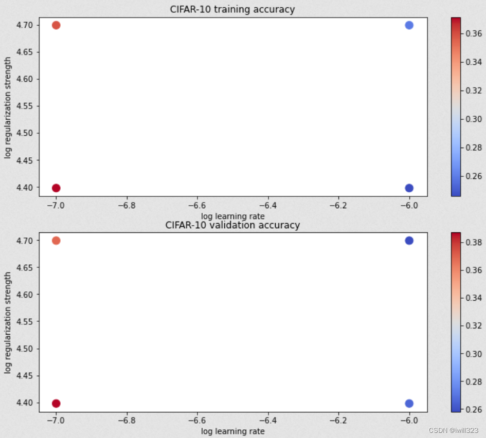
测试准确率
# Evaluate the best svm on test set
y_test_pred = best_svm.predict(X_test)
test_accuracy = np.mean(y_test == y_test_pred)
print('linear SVM on raw pixels final test set accuracy: %f' % test_accuracy)
可视化权重
# Visualize the learned weights for each class.
# Depending on your choice of learning rate and regularization strength, these may
# or may not be nice to look at.
w = best_svm.W[:-1,:] # strip out the bias
w = w.reshape(32, 32, 3, 10)
w_min, w_max = np.min(w), np.max(w)
classes = ['plane', 'car', 'bird', 'cat', 'deer', 'dog', 'frog', 'horse', 'ship', 'truck']
for i in range(10):plt.subplot(2, 5, i + 1)# Rescale the weights to be between 0 and 255wimg = 255.0 * (w[:, :, :, i].squeeze() - w_min) / (w_max - w_min)plt.imshow(wimg.astype('uint8'))plt.axis('off')plt.title(classes[i])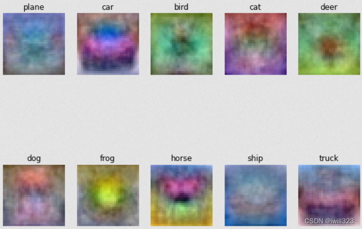
值得注意的地方
赋值
>>a = np.array([[1,2,3],[4,5,6]])
>>b = np.array([-1,-1])
>>print(b.shape)
(2,)
>>a[:,0] = b
>>print(a)
[[-1 2 3][-1 5 6]]
randrange
>>print(randrange(10))
3
np.arange
a = np.arange(8)
>>print(a)
>>print(np.random.choice(a,3))
>>print(np.random.choice(a,3))
>>print(np.random.choice(a,3))
[0 1 2 3 4 5 6 7]
[6 0 0]
[7 5 4]
[4 3 4]
np.random.choice
一般做法是事先将所有训练数据随机打乱,然后按指定的批次大小,按序生成 mini-batch。这样每个 mini-batch 均有一个索引号,比如此例可以是 0, 1, 2, ... , 99,然后用索引号可以遍历所有的 mini-batch。遍历一次所有数据,就称为一个epoch。请注意,本节中的mini-batch 每次都是用np.random.choice随机选择的,所以不一定每个数据都会被看到。
>>index = list(range(10))
>>print(np.random.choice(index,6, replace=False))
[4 7 9 8 1 2]
>>print(np.random.choice(5, 3, replace=False))
[3 3 0]
replace : Whether the sample is with or without replacement. Default is True, meaning that a value of ``a`` can be selected multiple times.
打乱数据可以使用random.shuffle或者np.random.permutation
np.random.permutation
>>idx = np.random.permutation(10)
>>print(idx)
>>a = list(range(10))
>>a = np.random.permutation(a)
>>print(a)
random.shuffle
>>ind = list(range(10))
>>random.shuffle(ind)
>>print(ind)
[2, 9, 6, 5, 0, 4, 3, 8, 1, 7]
>># print(random.shuffle(10)) 报错
>>index = torch.arange(10) # tensor([0, 1, 2, 3, 4, 5, 6, 7, 8, 9])
>>random.shuffle(list(index))
>>print(index) # 打乱的是list(index), 和index没有关系
tensor([0, 1, 2, 3, 4, 5, 6, 7, 8, 9])
>>indices = list(index)
>>random.shuffle(indices)
>>print(indices)
[tensor(3), tensor(4), tensor(8), tensor(5), tensor(2), tensor(9), tensor(6), tensor(7), tensor(1), tensor(0)]
>>random.shuffle(index.numpy())
>>print(index)
tensor([9, 1, 4, 3, 2, 0, 5, 7, 8, 6])
可以使用以下函数获取batch数据
def data_iter(batch_size, features, labels):num_examples = len(features)indices = list(range(num_examples))# 这些样本是随机读取的,没有特定的顺序random.shuffle(indices)for i in range(0, num_examples, batch_size):batch_indices = torch.tensor(indices[i: min(i + batch_size, num_examples)])yield features[batch_indices], labels[batch_indices]用到了yield:彻底理解Python中的yield - Ellisonzhang - 博客园
- 通常的for…in…循环中,in后面是一个数组,这个数组就是一个可迭代对象,类似的还有链表,字符串,文件。它可以是mylist
= [1, 2, 3],也可以是mylist = [x*x for x in range(3)]。 它的缺陷是所有数据都在内存中,如果有海量数据的话将会非常耗内存。 - 生成器是可以迭代的,但只可以读取它一次。因为用的时候才生成。比如 mygenerator = (x*x for x in
range(3)),注意这里用到了(),它就不是数组,而上面的例子是[]。 - 生成器(generator)能够迭代的关键是它有一个next()方法,工作原理就是通过重复调用next()方法,直到捕获一个异常。
mygenerator = (x*x for x in range(3)) print(next(mygenerator)) print(next(mygenerator)) # 0 # 1 - 带有 yield 的函数不再是一个普通函数,而是一个生成器generator,可用于迭代,工作原理同上。
- yield 是一个类似 return 的关键字,迭代一次遇到yield时就返回yield后面的值。重点是:下一次迭代时,从上一次迭代遇到的yield后面的代码开始执行。
- 简要理解:yield就是 return 返回一个值,并且记住这个返回的位置,下次迭代就从这个位置后开始。
- 带有yield的函数不仅仅只用于for循环中,而且可用于某个函数的参数,只要这个函数的参数允许迭代参数。比如array.extend函数,它的原型是array.extend(iterable)。
- send(msg)与next()的区别在于send可以传递参数给yield表达式,这时传递的参数会作为yield表达式的值,而yield的参数是返回给调用者的值。——换句话说,就是send可以强行修改上一个yield表达式值。比如函数中有一个yield赋值,a
= yield 5,第一次迭代到这里会返回5,a还没有赋值。第二次迭代时,使用.send(10),那么,就是强行修改yield 5表达式的值为10,本来是5的,那么a=10 - send(msg)与next()都有返回值,它们的返回值是当前迭代遇到yield时,yield后面表达式的值,其实就是当前迭代中yield后面的参数。
- 第一次调用时必须先next()或send(None),否则会报错,send后之所以为None是因为这时候没有上一个yield(根据第8条)。可以认为,next()等同于send(None)。
可以在for循环中,通过data_iter()取出数据,进行各种操作
for X, y in data_iter(batch_size, features, labels):print(X, '\n', y)breakdata_iter函数要求我们将所有数据加载到内存中,并执行大量的随机内存访问,执行效率很低。 在深度学习框架中实现的内置迭代器效率要高得多, 它可以处理存储在文件中的数据和数据流提供的数据


![[机器学习] 支持向量机通俗导论节选(一)](https://img-blog.csdn.net/20131111155205109)