神经网络的学习步骤如下所示:
步骤1(mini-batch)
从训练数据中随机选出一部分数据,目标是减小mini-batch的损失函数的值
步骤2(计算梯度)
为了减小mini-batch的损失函数的值,需要求出各个权重参数的梯度
步骤3(更新参数)
将权重参数沿梯度方向进行微小更新.
步骤4(重复)
重复步骤1、步骤2、步骤3。
这里因为使用的数据是随机选择的mini batch数据,所以称为随机梯度下降法(stochastic gradient descent)。深度学习的很多框架中,随机梯度下降法一般由一个名为SGD的函数来实现, SGD来源于随机梯度下降法的英文名称的首字母。
下面,来实现手写数字识别的神经网络。这里以2层神经网(隐藏层为1层的网络)为对象,使用MNIST数据集进行学习。
首先,下面看这个名为TwoLayerNet的类
# coding: utf-8
import sys, os
sys.path.append(os.pardir)  # 为了导入父目录的文件而进行的设定
from common.functions import *
from common.gradient import numerical_gradientclass TwoLayerNet:def __init__(self, input_size, hidden_size, output_size, weight_init_std=0.01):# 初始化权重# 保存神经网络的参数的字典型变量(实例变量)self.params = {}self.params['W1'] = weight_init_std * np.random.randn(input_size, hidden_size)self.params['b1'] = np.zeros(hidden_size)self.params['W2'] = weight_init_std * np.random.randn(hidden_size, output_size)self.params['b2'] = np.zeros(output_size)# 进行识别(推理)def predict(self, x):W1, W2 = self.params['W1'], self.params['W2']b1, b2 = self.params['b1'], self.params['b2']a1 = np.dot(x, W1) + b1z1 = sigmoid(a1)a2 = np.dot(z1, W2) + b2y = softmax(a2)return y# x:输入数据, t:监督数据def loss(self, x, t):y = self.predict(x)return cross_entropy_error(y, t)# 计算识别精度def accuracy(self, x, t):y = self.predict(x)y = np.argmax(y, axis=1)t = np.argmax(t, axis=1)accuracy = np.sum(y == t) / float(x.shape[0])return accuracy# x:输入数据, t:监督数据def numerical_gradient(self, x, t):loss_W = lambda W: self.loss(x, t)# 保存梯度的字典型变量grads = {}grads['W1'] = numerical_gradient(loss_W, self.params['W1'])grads['b1'] = numerical_gradient(loss_W, self.params['b1'])grads['W2'] = numerical_gradient(loss_W, self.params['W2'])grads['b2'] = numerical_gradient(loss_W, self.params['b2'])return gradsdef gradient(self, x, t):W1, W2 = self.params['W1'], self.params['W2']b1, b2 = self.params['b1'], self.params['b2']grads = {}batch_num = x.shape[0]# forwarda1 = np.dot(x, W1) + b1z1 = sigmoid(a1)a2 = np.dot(z1, W2) + b2y = softmax(a2)# backwarddy = (y - t) / batch_numgrads['W2'] = np.dot(z1.T, dy)grads['b2'] = np.sum(dy, axis=0)da1 = np.dot(dy, W2.T)dz1 = sigmoid_grad(a1) * da1grads['W1'] = np.dot(x.T, dz1)grads['b1'] = np.sum(dz1, axis=0)return grads
mini-batch的实现
神经网络的学习的实现使用的是前面介绍过的mini-batch学习。下面,就以TwoLayerNet类为对象,使用MNIST数据集进行学习
# coding: utf-8
import sys, os
sys.path.append(os.pardir)  # 为了导入父目录的文件而进行的设定
import numpy as np
import matplotlib.pyplot as plt
from dataset.mnist import load_mnist
from two_layer_net import TwoLayerNet# 读入数据
(x_train, t_train), (x_test, t_test) = load_mnist(normalize=True, one_hot_label=True)network = TwoLayerNet(input_size=784, hidden_size=50, output_size=10)iters_num = 10000  # 适当设定循环的次数
train_size = x_train.shape[0]
batch_size = 100
learning_rate = 0.1train_loss_list = []
train_acc_list = []
test_acc_list = []iter_per_epoch = max(train_size / batch_size, 1)for i in range(iters_num):# 获取mini-batchbatch_mask = np.random.choice(train_size, batch_size)x_batch = x_train[batch_mask]t_batch = t_train[batch_mask]# 计算梯度#grad = network.numerical_gradient(x_batch, t_batch)grad = network.gradient(x_batch, t_batch)# 更新参数for key in ('W1', 'b1', 'W2', 'b2'):network.params[key] -= learning_rate * grad[key]#记录学习过程loss = network.loss(x_batch, t_batch)train_loss_list.append(loss)# 计算每个epoch的识别精度if i % iter_per_epoch == 0:train_acc = network.accuracy(x_train, t_train)test_acc = network.accuracy(x_test, t_test)train_acc_list.append(train_acc)test_acc_list.append(test_acc)print("train acc, test acc | " + str(train_acc) + ", " + str(test_acc))# 绘制图形
markers = {'train': 'o', 'test': 's'}
x = np.arange(len(train_acc_list))
plt.plot(x, train_acc_list, label='train acc')
plt.plot(x, test_acc_list, label='test acc', linestyle='--')
plt.xlabel("epochs")
plt.ylabel("accuracy")
plt.ylim(0, 1.0)
plt.legend(loc='lower right')
plt.show()
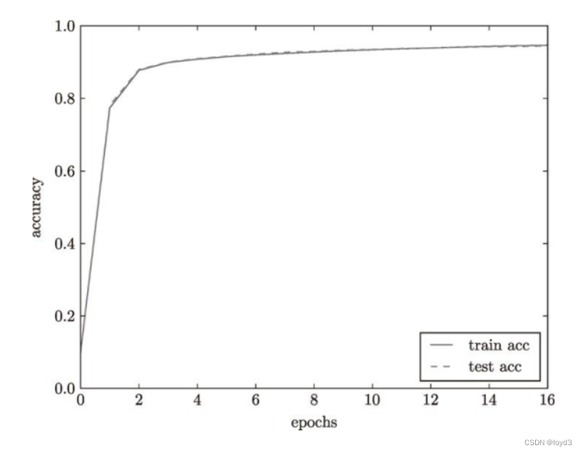
神经网络的学习中,必须确认是否能够正确识别训练数据以外的其他数据,即确认是否会发生过拟合。过拟合是指,虽然训练数据中的数字图像被正确辨别,但是不在训练数据中的数字图像却无法被识别的现象。
神经网络学习的最初目标是掌握泛化能力,因此,要评价神经网络的泛化能力,就必须使用不包含在训练数据中的数据。所以在进行学习过程中,要定期地对训练数据和测试数据记录识别精度。这里,每经过一个epoch,都会记录下训练数据和测试数据的识别精度。
epoch是一个单位。一个epoch表示学习中所有训练数据均被使用一次时的更新次数。比如,对于10000笔训练数据,用大小为100笔数据的mini-batch进行学习时,重复随机梯度下降法100次有的训练数据就都被“看过”了。此时,100次就是一个epoch
把从上面的代码中得到的结果用图标表示的话,如下图: