导航
- Bayesian Linear Regression
- Gibbs Sampling
- Derving a Gibbs sampler
- Update for β 0 \beta_0 β0
- Update for β 1 \beta_1 β1
- Update for τ \tau τ
- Synthetic data
- Gibbs sampler
- code downlaod
- References
Bayesian Linear Regression
考虑只有一个自变量(independent variable)的线性回归的情况,拟合数据对 ( y i , x i ) , i = 1 , 2 , … , N (y_i, x_i), i=1,2,\dots, N (yi,xi),i=1,2,…,N,需要找出后验分布中的截距(intercept) β 0 \beta_0 β0和斜率/梯度(gradient)以及精度 τ \tau τ(方差的倒数,the reciprocal of the variance),模型可以表示为
y i ∼ N ( β 0 + β 1 x i , 1 / τ ) y_i\sim\mathcal{N}(\beta_0+\beta_1x_i, 1/\tau) yi∼N(β0+β1xi,1/τ)
或者等价的
y i = β 0 + β 1 x i + ε , ε ∼ N ( 0 , 1 / τ ) y_i=\beta_0+\beta_1x_i+\varepsilon, \varepsilon\sim\mathcal{N}(0, 1/\tau) yi=β0+β1xi+ε,ε∼N(0,1/τ)
模型的似然函数可以被表示为 N N N个i.i.d观测点的乘积
L ( y 1 , … , y N , x 1 , x 2 , … , x N ∣ β 0 , β 1 , τ ) = ∏ i = 1 N N ( β 0 + β 1 x i , 1 / τ ) L(y_1, \dots, y_N, x_1, x_2, \dots, x_N\mid\beta_0, \beta_1, \tau)=\prod_{i=1}^N\mathcal{N}(\beta_0+\beta_1x_i, 1/\tau) L(y1,…,yN,x1,x2,…,xN∣β0,β1,τ)=i=1∏NN(β0+β1xi,1/τ)
希望设置 β 0 , β 1 , τ \beta_0, \beta_1, \tau β0,β1,τ得到共轭先验, conjugate priors
{ β 0 ∼ N ( μ 0 , 1 / τ 0 ) β 1 ∼ N ( μ 1 , 1 / τ 1 ) τ ∼ Γ ( α , β ) \left\{ \begin{aligned} &\beta_0\sim \mathcal{N}(\mu_0, 1/\tau_0)\\ &\beta_1\sim \mathcal{N}(\mu_1, 1/\tau_1)\\ &\tau\sim \Gamma(\alpha, \beta) \end{aligned} \right. ⎩⎪⎨⎪⎧β0∼N(μ0,1/τ0)β1∼N(μ1,1/τ1)τ∼Γ(α,β)
Gibbs Sampling
吉布斯采样的工作流程如下,假设我们有两个参数 θ 1 \theta_1 θ1和 θ 2 \theta_2 θ2以及一些数据 x x x,目标是找到后验分布 p ( θ 1 , θ 2 ∣ x ) p(\theta_1, \theta_2\mid x) p(θ1,θ2∣x).
To do this in a
Gibbs sampling regime, we need to work out the conditional distributions p ( θ 1 ∣ θ 1 , x ) p(\theta_1\mid \theta_1, x) p(θ1∣θ1,x) and p ( θ 2 ∣ θ 1 , x ) p(\theta_2\mid \theta_1, x) p(θ2∣θ1,x).
采样算法流程如下:
- 选择初始参数 θ 2 ( i + 1 ) \theta_2^{(i+1)} θ2(i+1)
- 采样 θ 1 ( i + 1 ) ∼ p ( θ 1 ∣ θ 2 ( i ) , x ) \theta_1^{(i+1)}\sim p(\theta_1\mid \theta_2^{(i)}, x) θ1(i+1)∼p(θ1∣θ2(i),x)
- 采样 θ 2 i + 1 ∼ p ( θ 2 ∣ θ 1 ( i + 1 ) , x ) \theta_2^{i+1}\sim p(\theta_2\mid\theta_1^{(i+1)}, x) θ2i+1∼p(θ2∣θ1(i+1),x)
流程重复 K K K轮,可以采集到 K K K个样本.
The key thing to remember in Gibbs sampling is to always use the most recent parameter values for all samples (e.g. sample θ 2 ( i + 1 ) ∼ p ( θ 2 ∣ θ 1 ( i + 1 ) , x ) \theta_2^{(i+1)}\sim p(\theta_2\mid \theta_1^{(i+1)}, x) θ2(i+1)∼p(θ2∣θ1(i+1),x) and
notθ 2 i + 1 ∼ p ( θ 2 ∣ θ 1 ( i ) , x ) \theta_2^{i+1}\sim p(\theta_2\mid \theta_1^{(i)}, x) θ2i+1∼p(θ2∣θ1(i),x) provided θ 1 ( i + 1 ) \theta_1^{(i+1)} θ1(i+1) has already been sampled).
The massive advantage of Gibbs sampling over other MCMC methods (namely Metropolis-Hastings) is that no tuning parameters are required.
Derving a Gibbs sampler
推导步骤如下
- Write down the posterior conditional density in log-form
- Throw away all terms that don’t depend on the current sampling variable
- Pretend this is the density for your variable of interest and all other variables are fixed. What distribution does the log-density remind of?
Update for β 0 \beta_0 β0
由贝叶斯公式可以得到
p ( β 0 ∣ β 1 , τ , y , x ) ∝ p ( y , x ∣ β 0 , β 1 , τ ) p ( β 0 ) p(\beta_0\mid \beta_1, \tau, y, x)\propto p(y, x \mid \beta_0, \beta_1, \tau)p(\beta_0) p(β0∣β1,τ,y,x)∝p(y,x∣β0,β1,τ)p(β0)
其中 p ( y , x ∣ β 0 , β 1 , τ ) p(y, x\mid \beta_0, \beta_1, \tau) p(y,x∣β0,β1,τ)是似然函数.
如果变量 x x x服从期望为 μ \mu μ,精度为 τ \tau τ的正态分布,关于 x x x的对数项(the log-dependence on x)为
τ 2 ( x − μ ) 2 ∝ − τ 2 x 2 + τ μ x \frac{\tau}{2}(x-\mu)^2\propto -\frac{\tau}{2}x^2+\tau\mu x 2τ(x−μ)2∝−2τx2+τμx
对数形式下关于 β 0 \beta_0 β0的项为
− τ 0 2 ( β 0 − μ 0 ) 2 − τ 2 ∑ i = 1 N ( y i − β 0 − β 1 x i ) 2 -\frac{\tau_0}{2}(\beta_0-\mu_0)^2-\frac{\tau}{2}\sum_{i=1}^N(y_i-\beta_0-\beta_1x_i)^2 −2τ0(β0−μ0)2−2τi=1∑N(yi−β0−β1xi)2
Although it is perhaps not obvious, this expression is quadratic in β 0 \beta_0 β0, meaning the conditional sampling density for β 0 \beta_0 β0 will also be normal. A bit of algebra(dropping all terms that do not involve β 0 \beta_0 β0) is
− τ 0 2 β 0 2 + τ 0 μ 0 β 0 − τ 2 N β 0 2 − τ ∑ i = 1 N ( y i − β 1 x i ) β 0 -\frac{\tau_0}{2}\beta_0^2+\tau_0\mu_0\beta_0-\frac{\tau}{2}N\beta_0^2-\tau\sum_{i=1}^N(y_i-\beta_1x_i)\beta_0 −2τ0β02+τ0μ0β0−2τNβ02−τi=1∑N(yi−β1xi)β0
即可以知道
β 0 \beta_0 β0的系数为 τ 0 μ 0 + τ ∑ i ( y i − β 1 x i ) \tau_0\mu_0+\tau\sum_i(y_i-\beta_1x_i) τ0μ0+τ∑i(yi−β1xi)
β 0 2 \beta_0^2 β02的系数为 − τ 0 2 − τ 2 N -\frac{\tau_0}{2}-\frac{\tau}{2}N −2τ0−2τN
表示 β 0 \beta_0 β0的条件采样分布(conditional sampling distribution)为
β 0 ∣ β 1 , τ , τ 0 , μ 0 , x , y ∼ N ( τ 0 μ 0 + τ ∑ i ( y i − β 1 x i ) τ 0 + τ N , 1 / ( τ 0 + τ N ) ) \beta_0\mid\beta_1,\tau, \tau_0,\mu_0,x,y\sim\mathcal{N}\bigg(\frac{\tau_0\mu_0+\tau\sum_i(y_i-\beta_1x_i)}{\tau_0+\tau N}, 1/(\tau_0+\tau N)\bigg) β0∣β1,τ,τ0,μ0,x,y∼N(τ0+τNτ0μ0+τ∑i(yi−β1xi),1/(τ0+τN))
def sample_beta_0(y, x, beta_1, tau, mu_0, tau_0):assert len(x)==len(y)N = len(y)precision=tau_0 + tau*Nmean = tau_0*mu_0+tau*np.sum(y-beta_1*x)mean /= precisionreturn random.normal(mean, 1/np.sqrt(precision)) # 得到beta_0采样
Update for β 1 \beta_1 β1
条件对数后验方程中关于 β 1 \beta_1 β1的项为
τ 1 2 ( β 1 − μ 1 ) 2 − τ 2 ∑ i = 1 N ( y i − β 0 − β 1 x i ) 2 \frac{\tau_1}{2}(\beta_1-\mu_1)^2-\frac{\tau}{2}\sum_{i=1}^N(y_i-\beta_0-\beta_1x_i)^2 2τ1(β1−μ1)2−2τi=1∑N(yi−β0−β1xi)2
展开得到
− τ 1 2 β 1 2 + τ 1 μ 1 β 1 − τ 2 ∑ i x i 2 β 1 2 + τ ∑ i ( y i − β 0 ) x i β 1 -\frac{\tau_1}{2}\beta_1^2+\tau_1\mu_1\beta_1-\frac{\tau}{2}\sum_ix_i^2\beta_1^2+\tau\sum_i(y_i-\beta_0)x_i\beta_1 −2τ1β12+τ1μ1β1−2τi∑xi2β12+τi∑(yi−β0)xiβ1
β 1 \beta_1 β1的系数为 τ 1 μ 1 + τ ∑ i ( y i − β 0 ) x i \tau_1\mu_1+\tau\sum_i(y_i-\beta_0)x_i τ1μ1+τ∑i(yi−β0)xi, β 1 2 \beta_1^2 β12的系数为 − τ 1 2 − τ 2 ∑ i x i 2 -\frac{\tau_1}{2}-\frac{\tau}{2}\sum_ix_i^2 −2τ1−2τ∑ixi2,所以 β 1 \beta_1 β1的条件采样密度为
β 0 ∣ β 1 , τ , τ 0 , μ 0 , x , y ∼ N ( τ 0 μ 0 + τ ∑ i ( y i − β 1 x i ) τ 0 + τ N , 1 / ( τ 0 + τ N ) ) \beta_0\mid\beta_1,\tau, \tau_0,\mu_0, x, y\sim \mathcal{N}\bigg(\frac{\tau_0\mu_0+\tau\sum_i(y_i-\beta_1x_i)}{\tau_0+\tau N}, 1/(\tau_0+\tau N) \bigg) β0∣β1,τ,τ0,μ0,x,y∼N(τ0+τNτ0μ0+τ∑i(yi−β1xi),1/(τ0+τN))
def sample_beta_1(y, x, beta_0, tau, mu_1, tau_1):assert len(x)==len(y)precision=tau_1+tau*np.sum(x*x)mean=tau_1*mu_1+tau*np.sum((y-beta_0)*x)mean/=precisionreturn random.normal(mean, 1/np.sqrt(precision))
Update for τ \tau τ
需要在non-Gaussian distributions下完成对 τ \tau τ值得更新,引入 Γ ( α , β ) \Gamma(\alpha, \beta) Γ(α,β)分布
p ( x ; α , β ) ∝ ( α − 1 ) log x − β x p(x; \alpha, \beta)\propto (\alpha-1)\log x-\beta x p(x;α,β)∝(α−1)logx−βx
带回方程得到
p ( τ ∣ β 0 , β 1 , y , x ) ∝ p ( y , x ∣ β 0 ) p ( τ ) p(\tau\mid \beta_0, \beta_1, y, x)\propto p(y, x\mid \beta_0)p(\tau) p(τ∣β0,β1,y,x)∝p(y,x∣β0)p(τ)
密度函数为
∏ i = 1 N N ( y i ∣ β 0 + β 1 x i ; 1 / τ ) × Γ ( τ ∣ α , β ) \prod_{i=1}^N \mathcal{N}(y_i\mid \beta_0+\beta_1x_i; 1/\tau)\times \Gamma(\tau\mid \alpha, \beta) i=1∏NN(yi∣β0+β1xi;1/τ)×Γ(τ∣α,β)
有概率密度函数的对数形式可以知道
N 2 log τ − τ 2 ∑ i ( y i − β 0 − β 1 x i ) 2 + ( α − 1 ) log τ − β τ \frac{N}{2}\log\tau-\frac{\tau}{2}\sum_i(y_i-\beta_0-\beta_1x_i)^2+(\alpha-1)\log\tau-\beta\tau 2Nlogτ−2τi∑(yi−β0−β1xi)2+(α−1)logτ−βτ
根据系数可以知道
τ ∣ β 0 , β 1 , α , β , x , y ∼ Γ ( α + N 2 , β + ∑ i ( y i − β 0 − β 1 x i ) 2 2 ) \tau\mid\beta_0, \beta_1, \alpha, \beta, x, y\sim \Gamma(\alpha+\frac{N}{2}, \beta+\sum_i\frac{(y_i-\beta_0-\beta_1x_i)^2}{2}) τ∣β0,β1,α,β,x,y∼Γ(α+2N,β+i∑2(yi−β0−β1xi)2)
Synthetic data
设置 β 0 = − 1 , β 1 = 2 , τ = 1 \beta_0=-1, \beta_1=2, \tau=1 β0=−1,β1=2,τ=1为真实参数
def synthetic_data():beta_0_true=-1beta_1_true=2tau_true=1N=50x=random.uniform(low=0, high=4, size=N)y=random.normal(beta_0_true+beta_1_true*x, 1/np.sqrt(tau_true))syn_plt=plt.plot(x, y, 'o')plt.xlabel('x(uni. dist.)')plt.ylabel('y(normal dist.)')plt.grid(True)plt.show()

Gibbs sampler
设置 β 0 , β 1 \beta_0,\beta_1 β0,β1服从先验为 N ( 0 , 1 ) \mathcal{N}(0, 1) N(0,1), τ \tau τ服从先验 Γ ( 2 , 1 ) \Gamma(2, 1) Γ(2,1)
x, y, N = synthetic_data()# 设置参数起点
init={'beta_0':0, 'beta_1':0, 'tau':2}
# 超参数
hypers={'mu_0': 0, 'tau_0':1, 'mu_1':0, 'tau_1':1, 'alpha':2, 'beta': 1}def gibbs(y, x, iters, init, hypers):assert len(x)==len(y)beta_0, beta_1, tau=init['beta_0'], init['beta_1'], init['tau']param_rec = np.zeros((iters, 3)) # 记录参数的变化for i in range(iters):beta_0=sample_beta_0(y, x, beta_1, tau, hypers['mu_0'], hypers['tau_0'])beta_1=sample_beta_1(y, x, beta_0, tau, hypers['mu_1'], hypers['tau_1'])tau = sample_tau(y, x, beta_0, beta_1, hypers['alpha'], hypers['beta'], N)param_rec[i, :]=np.array((beta_0, beta_1, tau))param_rec = DataFrame(param_rec)param_rec.columns=['beta_0', 'beta_1', 'tau']return param_recdef params():iters=1000 # 设置迭代轮数param_rec = gibbs(y, x, iters, init, hypers)it = [*range(1, iters+1)]beta_0 = param_rec['beta_0'].valuesbeta_1 = param_rec['beta_1'].valuestau = param_rec['tau'].valuesplt.plot(it, beta_0, '-.', color='b', linewidth=1, label='beta_0')plt.plot(it, beta_1, '-.', color='r', linewidth=1, label='beta_1')plt.plot(it, tau, '-.', color='g', linewidth=1, label='tau')plt.grid(True)plt.legend(loc='best')plt.show()params()
得到采样参数变化路径如下
 从采样结果可以发现,开始采样时,参数波动比较大,后来逐渐在真实值附近波动.
Even if it is obvious that the variables converge early it is convention to define a
burn-inperiod where we assume the parameters are still converging, which is typically half of iterations. Therefore, we could check the final 500 iterations calledtrace_burnt
考察采样后半部分的参数
def trace_burnt():iters=1000param_rec = gibbs(y, x, iters, init, hypers)[500:-1]print(param_rec.median()) # 采样得到参数的中位数print(param_rec.std()) # 采样得到参数的标准差hist_plot = param_rec.hist(bins=30, layout=(1, 3))plt.show()

code downlaod
Gibbs sampling python code
References
seaborn画图
Bayesian Data Analysis
Gibbs Sampling
Gibbs sampling for Bayesian linear regression
Markov Chain Monte Carlo(MCMC)
Gibbs采样完整解析与理解