一、理论基础

高斯模型就是用高斯概率密度函数（正态分布曲线）精确地量化事物，将一个事物分解为若干的基于高斯概率密度函数（正态分布曲线）形成的模型。对图像背景建立高斯模型的原理及过程：图像灰度直方图反映的是图像中某个灰度值出现的频次，也可以以为是图像灰度概率密度的估计。如果图像所包含的目标区域和背景区域相差比较大，且背景区域和目标区域在灰度上有一定的差异，那么该图像的灰度直方图呈现双峰-谷形状，其中一个峰对应于目标，另一个峰对应于背景的中心灰度。对于复杂的图像，尤其是医学图像，一般是多峰的。通过将直方图的多峰特性看作是多个高斯分布的叠加，可以解决图像的分割问题。在智能监控系统中，对于运动目标的检测是中心内容，而在运动目标检测提取中，背景目标对于目标的识别和跟踪至关重要。而建模正是背景目标提取的一个重要环节。

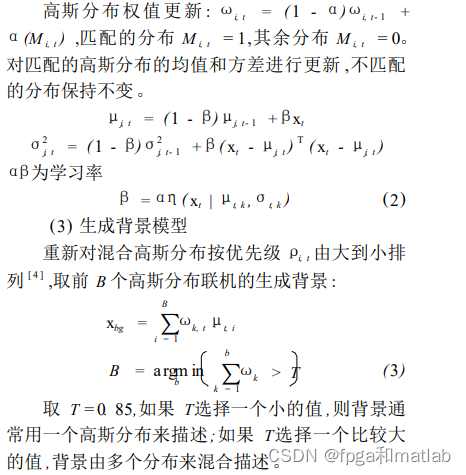
混合高斯模型使用K（基本为3到5个）个高斯模型来表征图像中各个像素点的特征,在新一帧图像获得后更新混合高斯模型, 用当前图像中的每个像素点与混合高斯模型匹配,如果成功则判定该点为背景点, 否则为前景点。通观整个高斯模型，主要是有方差和均值两个参数决定，对均值和方差的学习，采取不同的学习机制,将直接影响到模型的稳定性、精确性和收敛性。由于我们是对运动目标的背景提取建模，因此需要对高斯模型中方差和均值两个参数实时更新。为提高模型的学习能力,改进方法对均值和方差的更新采用不同的学习率;为提高在繁忙的场景下,大而慢的运动目标的检测效果,引入权值均值的概念,建立背景图像并实时更新,然后结合权值、权值均值和背景图像对像素点进行前景和背景的分类。

到这里为止，混合高斯模型的建模基本完成，我在归纳一下其中的流程，首先初始化预先定义的几个高斯模型，对高斯模型中的参数进行初始化，并求出之后将要用到的参数。其次，对于每一帧中的每一个像素进行处理，看其是否匹配某个模型，若匹配，则将其归入该模型中，并对该模型根据新的像素值进行更新，若不匹配，则以该像素建立一个高斯模型，初始化参数，代理原有模型中最不可能的模型。最后选择前面几个最有可能的模型作为背景模型，为背景目标提取做铺垫。

混合高斯模型法是背景提取领域中比较常用的一种算法,这种方法通过对每一个像素点的亮度用若干个高斯模型来建模,使该方法在进行背景提取的时候具有一定的场景适应能力,可以克服其他背景提取算法(如:多帧平均法,统计中值法等)无法适应环境变化的缺点.对于多峰高斯分布模型，图像的每一个像素点按不同权值的多个高斯分布的叠加来建模，每种高斯分布对应一个可能产生像素点所呈现颜色的状态，各个高斯分布的权值和分布参数随时间更新。

当处理彩色图像时，假定图像像素点R、G、B三色通道相互独立并具有相同的方差。对于随机变量X的观测数据集{x1,x2,…,xN}，xt=(rt,gt,bt)为t时刻像素的样本，则单个采样点xt其服从的混合高斯分布概率密度函数：

所谓单高斯模型，就是用多维高斯分布概率来进行模式分类，其中μ用训练样本均值代替，Σ用样本方差代替，X为d维的样本向量。通过高斯概率公式就可以得出类别C属于正（负）样本的概率。而混合高斯模型（GMM）就是数据从多个高斯分布中产生的。每个GMM由K个高斯分布线性叠加而 P（x）=Σp(k)*p(x|k) 相当于对各个高斯分布进行加权（权系数越大，那么这个数据属于这个高斯分布的可能性越大）而在实际过程中，我们是在已知数据的前提下，对GMM进行参数估计，具体在这里即为图片训练一个合适的GMM模型。那么在前景检测中，我们会取静止背景（约50帧图像）来进行GMM参数估计，进行背景建模。分类域值官网取得0.7，经验取值0.7-0.75可调。这一步将会分离前景和背景，输出为前景二值掩码。

二、核心程序

.............................................................................% Now update the weights. Increment weight for the selected Gaussian (if any),% and decrement weights for all other Gaussians.   Weights = (1 - ALPHA) .* Weights + ALPHA .* matched_gaussian;% Adjust Mus and Sigmas for matching distributions.for kk = 1:Kpixel_matched = repmat(matched_gaussian(:, kk), 1, C);pixel_unmatched = abs(pixel_matched - 1); % Inverted and mutually exclusiveMu_kk = reshape(Mus(:, kk, :), D, C);Sigma_kk = reshape(Sigmas(:, kk, :), D, C);Mus(:, kk, :) = pixel_unmatched .* Mu_kk + ...pixel_matched .* (((1 - RHO) .* Mu_kk) + ...(RHO .* double(image)));% Get updated Mus; Sigmas is still unchangedMu_kk = reshape(Mus(:, kk, :), D, C); Sigmas(:, kk, :) = pixel_unmatched .* Sigma_kk + ...pixel_matched .* (((1 - RHO) .* Sigma_kk) + ...repmat((RHO .* sum((double(image) - Mu_kk) .^ 2, 2)), 1, C));       end% Maintain an indicator matrix of those components that were replaced because no component matched. replaced_gaussian = zeros(D, K); % Find those pixels which have no Gaussian that matchesmismatched = find(sum(matched_gaussian, 2) == 0);% A method that works well: Replace the component we            % are least confident in. This includes weight in the choice of % component.        for ii = 1:length(mismatched)[junk, index] = min(Weights(mismatched(ii), :) ./ sqrt(Sigmas(mismatched(ii), :, 1)));% Mark that this Gaussian will be replacedreplaced_gaussian(mismatched(ii), index) = 1;% With a distribution that has the current pixel as meanMus(mismatched(ii), index, :) = image(mismatched(ii), :);% And a relatively wide varianceSigmas(mismatched(ii), index, :) = ones(1, C) * INIT_VARIANCE;% Also set the weight to be relatively smallWeights(mismatched(ii), index) = INIT_MIXPROP;  end% Now renormalise the weights so they still sum to 1Weights = Weights ./ repmat(sum(Weights, 2), 1, K);active_gaussian = matched_gaussian + replaced_gaussian;%----------------------------------------------------------------------%--------------------------background Segment--------------------------% Find maximum weight/sigma per row. [junk, index] = sort(Weights ./ sqrt(Sigmas(:, :, 1)), 2, 'descend');% Record indeces of those each pixel's component we are most confident% in, so that we can display a single background estimate later. While % our model allows for a multi-modal background, this is a useful% visualisation when something goes wrong. best_background_gaussian = index(:, 1);linear_index = (index - 1) * D + repmat([1:D]', 1, K);weights_ordered = Weights(linear_index);for kk = 1:Kaccumulated_weights(:, kk) = sum(weights_ordered(:, 1:kk), 2);endbackground_gaussians(:, 2:K) = accumulated_weights(:, 1:(K-1)) < BACKGROUND_THRESH;background_gaussians(:, 1) = 1;            % The first will always be selected% Those pixels that have no active background Gaussian are considered forground. background_gaussians(linear_index) = background_gaussians;active_background_gaussian = active_gaussian & background_gaussians;foreground_pixels = abs(sum(active_background_gaussian, 2) - 1);foreground_map = reshape(sum(foreground_pixels, 2), HEIGHT, WIDTH);foreground_with_map_sequence(:, :, tt) = foreground_map;   %----------------------------------------------------------------------%---------------------Connected components-----------------------------objects_map = zeros(size(foreground_map), 'int32');object_sizes = [];object_positions = [];new_label = 1;[label_map, num_labels] = bwlabel(foreground_map, 8);for label = 1:num_labels object = (label_map == label);object_size = sum(sum(object));if(object_size >= COMPONENT_THRESH)%Component is big enough, mark itobjects_map = objects_map + int32(object * new_label);object_sizes(new_label) = object_size;[X, Y] = meshgrid(1:WIDTH, 1:HEIGHT);    object_x = X .* object;object_y = Y .* object;object_positions(:, new_label) = [sum(sum(object_x)) / object_size;sum(sum(object_y)) / object_size];new_label = new_label + 1;endendnum_objects = new_label - 1;%---------------------------Shadow correction--------------------------% Produce an image of the means of those mixture components which we are most% confident in using the weight/stddev tradeoff.index = sub2ind(size(Mus), reshape(repmat([1:D], C, 1), D * C, 1), ...reshape(repmat(best_background_gaussian', C, 1), D * C, 1), repmat([1:C]', D, 1));background = reshape(Mus(index), C, D);background = reshape(background', HEIGHT, WIDTH, C); background = uint8(background);background_sequence(:, :, :, tt) = background;background_hsv = rgb2hsv(background);image_hsv = rgb2hsv(image_sequence(:, :, :, tt));for i = 1:HEIGHTfor j = 1:WIDTH      if (objects_map(i, j)) && (abs(image_hsv(i,j,1) - background_hsv(i,j,1)) < 0.7)...&& (image_hsv(i,j,2) - background_hsv(i,j,2) < 0.25)...&& (0.85 <=image_hsv(i,j,3)/background_hsv(i,j,3) <= 0.95)shadow_mark(i, j) = 1;  elseshadow_mark(i, j) = 0;  end               end    endforeground_map_sequence(:, :, tt) = objects_map;
%     objecs_adjust_map = objects_map & (~shadow_mark);objecs_adjust_map = shadow_mark;foreground_map_adjust_sequence(:, :, tt) = objecs_adjust_map;    %----------------------------------------------------------------------
end
%--------------------------------------------------------------------------% -----------------------------Result display-------------------------------
figure;
while 1
for tt = 1:T
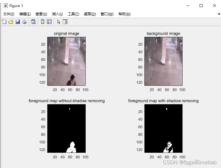
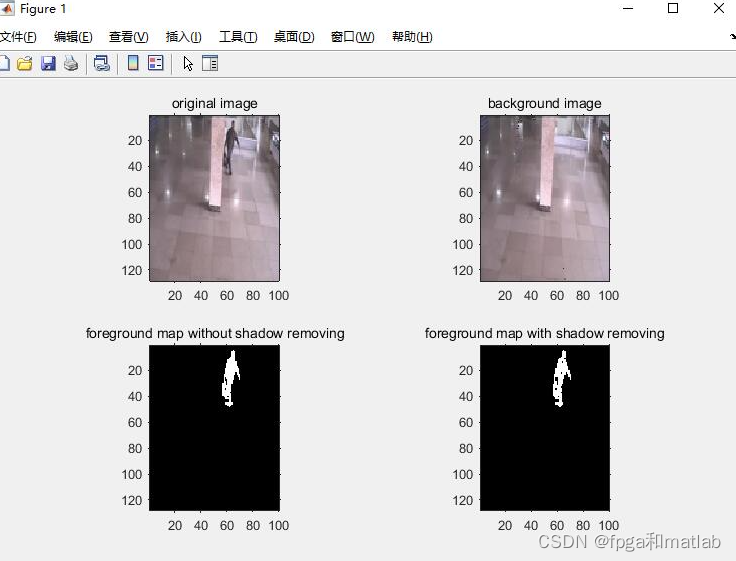
%   tt = 30;subplot(2,2,1),imshow(image_sequence(:, :, :, tt));title('original image');subplot(2,2,2),imshow(uint8(background_sequence(:, :, :, tt)));title('background image');subplot(2,2,3),imshow(foreground_map_sequence(:, :, tt)); title('foreground map without shadow removing');
%   subplot(2,2,4),imshow(uint8(background_sequence(:, :, :, tt)));subplot(2,2,4),imshow(foreground_map_adjust_sequence(:, :, tt));title('foreground map with shadow removing');drawnow;pause(0.1);
end
end
up141