单方程误差修正模型案例分析
数据的生成
set.seed(12345)
u<-rnorm(500)
x<-cumsum(u)
y<-x+u
E-G协整估计及检验
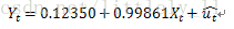
model.lm<-lm(y~x)
summary(model.lm)

Call:
lm(formula = y ~ x)Residuals:Min       1Q   Median       3Q      Max 
-2.65130 -0.65274  0.02012  0.60176  2.66642 Coefficients:Estimate Std. Error t value Pr(>|t|)    
(Intercept)  0.12350    0.10797   1.144    0.253    
x            0.99861    0.00333 299.924   <2e-16 ***
---
Signif. codes:  0 ‘***’ 0.001 ‘**’ 0.01 ‘*’ 0.05 ‘.’ 0.1 ‘ ’ 1Residual standard error: 0.991 on 498 degrees of freedom
Multiple R-squared:  0.9945,    Adjusted R-squared:  0.9945 
F-statistic: 8.995e+04 on 1 and 498 DF,  p-value: < 2.2e-16第一步建立协整关系，利用OLS法得到X和Y的协整回归方程:

提取协整回归残差

re.lm<-resid(model.lm)
协整检验，应用包urca
summary(ur.df(re.lm,type="none",selectlags="AIC"))

############################################### 
# Augmented Dickey-Fuller Test Unit Root Test # 
############################################### Test regression none Call:
lm(formula = z.diff ~ z.lag.1 - 1 + z.diff.lag)Residuals:Min       1Q   Median       3Q      Max 
-2.70068 -0.66375  0.03806  0.61796  2.65938 Coefficients:Estimate Std. Error t value Pr(>|t|)    
z.lag.1    -1.04076    0.06345 -16.404   <2e-16 ***
z.diff.lag  0.03986    0.04485   0.889    0.375    
---
Signif. codes:  0 ‘***’ 0.001 ‘**’ 0.01 ‘*’ 0.05 ‘.’ 0.1 ‘ ’ 1Residual standard error: 0.9916 on 496 degrees of freedom
Multiple R-squared:  0.5013,    Adjusted R-squared:  0.4993 
F-statistic: 249.3 on 2 and 496 DF,  p-value: < 2.2e-16Value of test-statistic is: -16.4041 Critical values for test statistics: 1pct  5pct 10pct
tau1 -2.58 -1.95  -1.62
dy<-diff(y)
dx<-diff(x)
error.term<-head(re.lm,-1)
data.ecm<-data.frame(dy=dy,dx=dx,error.term=error.term)
model.ecm<-lm(dy~dx+error.term,data=data.ecm)
summary(model.ecm)

Call:
lm(formula = dy ~ dx + error.term, data = data.ecm)Residuals:Min        1Q    Median        3Q       Max 
-0.043268 -0.008857 -0.001662  0.016696  0.035626 Coefficients:Estimate Std. Error  t value Pr(>|t|)    
(Intercept) -0.0823551  0.0008290   -99.34   <2e-16 ***
dx           1.9983047  0.0008346  2394.21   <2e-16 ***
error.term  -0.9999880  0.0008347 -1198.03   <2e-16 ***
---
Signif. codes:  0 ‘***’ 0.001 ‘**’ 0.01 ‘*’ 0.05 ‘.’ 0.1 ‘ ’ 1Residual standard error: 0.01846 on 496 degrees of freedom
Multiple R-squared:  0.9999,    Adjusted R-squared:  0.9999 
F-statistic: 3.585e+06 on 2 and 496 DF,  p-value: < 2.2e-16

第二步建立误差修正模型，估计结果为：

其中，误差校正项为:

误差校正系数为0.9999880.