论文下载
bib:
@inproceedings{chenduan2016infogan,author 		= {Xi Chen and Yan Duan and Rein Houthooft and John Schulman and Ilya Sutskever and Pieter Abbeel},title 		= {InfoGAN: Interpretable Representation Learning by Information Maximizing Generative Adversarial Nets},booktitle 	= {NIPS},year 		= {2016},pages 		= {2180--2188}
}
1. 摘要
This paper describes InfoGAN, an information-theoretic extension to the Generative Adversarial Network that is able to learn
disentangled representationsin a completely unsupervised manner. InfoGAN is a generative adversarial network that also maximizes the mutual information between a small subset of the latent variables and the observation. We derive a lower bound of themutual informationobjective that can be optimized efficiently. Specifically, InfoGAN successfully disentangles writing styles from digit shapes on the MNIST dataset, pose from lighting of 3D rendered images, and background digits from the central digit on the SVHN dataset. It also discovers visual concepts that include hair styles, presence/absence of eyeglasses, and emotions on the CelebA face dataset. Experiments show that InfoGAN learns interpretable representations that are competitive with representations learned by existing supervised methods.
本文描述了InfoGAN,它是生成对抗网络的一个信息论扩展,能够以完全无监督的方式学习
解耦表征。InfoGAN是一个生成式对抗网络,它也能最大化一个小子集的潜在变量与观测值之间的互信息。我们得到了一个可以有效优化的互信息目标的下界。具体来说,InfoGAN成功地从MNIST数据集的数字形状中分离出书写风格,从3D渲染图像的照明中分离出姿势,从SVHN数据集的中心数字中分离出背景数字。它还发现了CelebA脸部数据集上的视觉概念,包括发型、是否戴眼镜和情绪。实验表明,InfoGAN学习的可解释表示与现有的有监督学习方法学习的表示具有竞争性。
本文是一种GAN模型的变体,旨在学习一种可解释特征。
2. 前置知识
2.1 disentangled representations
Single latent units are sensitive to changes in single generative factors, while being relatively invariant to changes in other factors.
解耦表征学习是一个方向,意在获取一个表征,其中一个维度的变化对应于一个变化因子的变化, 而其他因子相对不变。关于disentangled representations, 可以参见博客。现在我的理解是,原本GAN对于一个潜在变量只能完成随机的生成任务,因为辨别器只能辨别生成器生成的图片是否为真实图片的二分类任务。在GAN的基础上,衍生出CGAN,即条件GAN,将标签带入生成。也就是辨别器不只是惩罚生成器不是真实图片的情况,还要惩罚生成图片不是对应标签的图片。按照现在的理解,InfoGAN更加进了一步,不只要控制生成图片的类别,还要控制生成图片的样式(style)。
2.2 mutual information
这里不涉及具体的数学解释,只是一个粗略的理解。互信息是一个随机变量由于已知另一个随机变量而减少的不肯定性。举个栗子,X=今天下雨,Y = 今天是阴天,那么已知道今天是阴天,那么X(今天下雨的概率)会增加,增加的量就是两个变量之间的互信息。由此可知,互信息只存在于两个非独立的随机变量中。Z=今天看论文,X与Z之间就没有互信息,每天都要看论文,与今天的天气无关🐶。
I ( X ; Y ) = ∑ x ∈ X ∑ y ∈ Y p ( x , y ) log p ( x , y ) p ( x ) p ( y ) (1) I(X; Y) = \sum_{x \in X}\sum_{y \in Y}p(x,y)\text{log}\frac{p(x,y)}{p(x)p(y)}\tag{1} I(X;Y)=x∈X∑y∈Y∑p(x,y)logp(x)p(y)p(x,y)(1)
3. 算法
-
standard GAN:
min G max D V ( D , G ) = E x ∼ p d a t a [ log ( D ( x ) ) ] + E z ∼ noise [ log ( 1 − D ( z ) ) ] (2) \min_{G}\max_{D}V(D, G) = \mathbb{E}_{x \sim p_{data}}[\log(D(x))] + \mathbb{E}_{z \sim {\text{noise}}}[\log(1- D(z))] \tag{2} GminDmaxV(D,G)=Ex∼pdata[log(D(x))]+Ez∼noise[log(1−D(z))](2) -
infoGAN:
min G max D V ( D , G ) − λ I ( c ; G ( z , c ) ) (3) \min_{G}\max_{D}V(D, G) - \lambda I(c; G(z, c))\tag{3} GminDmaxV(D,G)−λI(c;G(z,c))(3)
tips:
-
infoGAN不同的地方在于添加了一个互信息正则,旨在保证G的生成满足潜在变量c的语义,这个是在标准GAN中没有的(标准GAN是随机生成,没有具体语义)。
-
对于这个互信息正则才是这篇论文的工作核心。其实互信息只是其中一种方法,只是在这里用到了,说到底只要是能惩罚生成 G ( z , c ) G(z, c) G(z,c)与规定语义 c c c之间的不同就可以。

在博客中,我还找到上面这个图, 原论文中没有这个图,没有去探究出处。由此, Q Q Q就是设计互信息正则的关键。
Question:
- 特征信息是如何指定的?数字离散信息,数字表示的连续信息。
Answer:实际上是没有指定的,在训练的过程中是没有使用真实图片的标签的,可以理解为是一个无监督的学习过程。 - G和Q组成了一组编码解码器,Q企图从G生成的图片中获取c(带有信息的标签),实际上G和Q共享卷积层的模型参数。
- InfoGAN是一种Conditional GAN,也就是不是随机生成,想通过条件变量来控制生成。
4. 代码
这段是我找到的一个可以运行的代码,但是忘记了出处,侵权可以删除。
import argparse
import os
import numpy as np
import math
import itertoolsimport torchvision.transforms as transforms
from torchvision.utils import save_imagefrom torch.utils.data import DataLoader
from torchvision import datasets
from torch.autograd import Variableimport torch.nn as nn
import torch.nn.functional as F
import torch
import sysos.makedirs("images/static/", exist_ok=True)
os.makedirs("images/varying_c1/", exist_ok=True)
os.makedirs("images/varying_c2/", exist_ok=True)parser = argparse.ArgumentParser()
parser.add_argument("--n_epochs", type=int, default=200, help="number of epochs of training")
parser.add_argument("--batch_size", type=int, default=64, help="size of the batches")
parser.add_argument("--lr", type=float, default=0.0002, help="adam: learning rate")
parser.add_argument("--b1", type=float, default=0.5, help="adam: decay of first order momentum of gradient")
parser.add_argument("--b2", type=float, default=0.999, help="adam: decay of first order momentum of gradient")
parser.add_argument("--n_cpu", type=int, default=8, help="number of cpu threads to use during batch generation")
parser.add_argument("--latent_dim", type=int, default=62, help="dimensionality of the latent space")
parser.add_argument("--code_dim", type=int, default=2, help="latent code")
parser.add_argument("--n_classes", type=int, default=10, help="number of classes for dataset")
parser.add_argument("--img_size", type=int, default=32, help="size of each image dimension")
parser.add_argument("--channels", type=int, default=1, help="number of image channels")
parser.add_argument("--sample_interval", type=int, default=400, help="interval between image sampling")
opt = parser.parse_args()
print(opt)cuda = True if torch.cuda.is_available() else Falsedef weights_init_normal(m):classname = m.__class__.__name__if classname.find("Conv") != -1:torch.nn.init.normal_(m.weight.data, 0.0, 0.02)elif classname.find("BatchNorm") != -1:torch.nn.init.normal_(m.weight.data, 1.0, 0.02)torch.nn.init.constant_(m.bias.data, 0.0)# one-hot 编码
def to_categorical(y, num_columns):"""Returns one-hot encoded Variable"""y_cat = np.zeros((y.shape[0], num_columns))y_cat[range(y.shape[0]), y] = 1.0return Variable(FloatTensor(y_cat))class Generator(nn.Module):def __init__(self):super(Generator, self).__init__()input_dim = opt.latent_dim + opt.n_classes + opt.code_dimself.init_size = opt.img_size // 4  # Initial size before upsamplingself.l1 = nn.Sequential(nn.Linear(input_dim, 128 * self.init_size ** 2))self.conv_blocks = nn.Sequential(nn.BatchNorm2d(128),nn.Upsample(scale_factor=2),nn.Conv2d(128, 128, 3, stride=1, padding=1),nn.BatchNorm2d(128, 0.8),nn.LeakyReLU(0.2, inplace=True),nn.Upsample(scale_factor=2),nn.Conv2d(128, 64, 3, stride=1, padding=1),nn.BatchNorm2d(64, 0.8),nn.LeakyReLU(0.2, inplace=True),nn.Conv2d(64, opt.channels, 3, stride=1, padding=1),nn.Tanh(),)def forward(self, noise, labels, code):# [b, 62], [b,10], [b,2]gen_input = torch.cat((noise, labels, code), -1)out = self.l1(gen_input)# 重构成b个128*8*8的图out = out.view(out.shape[0], 128, self.init_size, self.init_size)# 然后进入卷积层,得到b个1*32*32的图片img = self.conv_blocks(out)return imgclass Discriminator(nn.Module):def __init__(self):super(Discriminator, self).__init__()def discriminator_block(in_filters, out_filters, bn=True):"""Returns layers of each discriminator block"""block = [nn.Conv2d(in_filters, out_filters, 3, 2, 1), nn.LeakyReLU(0.2, inplace=True), nn.Dropout2d(0.25)]if bn:block.append(nn.BatchNorm2d(out_filters, 0.8))return blockself.conv_blocks = nn.Sequential(*discriminator_block(opt.channels, 16, bn=False),*discriminator_block(16, 32),*discriminator_block(32, 64),*discriminator_block(64, 128),)# The height and width of downsampled imageds_size = opt.img_size // 2 ** 4# Output layers# Discriminator的最后一层self.adv_layer = nn.Sequential(nn.Linear(128 * ds_size ** 2, 1))# Classifier的最后一层self.aux_layer = nn.Sequential(nn.Linear(128 * ds_size ** 2, opt.n_classes), nn.Softmax())self.latent_layer = nn.Sequential(nn.Linear(128 * ds_size ** 2, opt.code_dim))def forward(self, img):out = self.conv_blocks(img)out = out.view(out.shape[0], -1)validity = self.adv_layer(out)label = self.aux_layer(out)latent_code = self.latent_layer(out)# c = [label, latent_code],即 [64*10,64*2]return validity, label, latent_code# Loss functions
adversarial_loss = torch.nn.MSELoss()
categorical_loss = torch.nn.CrossEntropyLoss()
continuous_loss = torch.nn.MSELoss()# Loss weights
lambda_cat = 1
lambda_con = 0.1# Initialize generator and discriminator
generator = Generator()
discriminator = Discriminator()if cuda:generator.cuda()discriminator.cuda()adversarial_loss.cuda()categorical_loss.cuda()continuous_loss.cuda()# Initialize weights
generator.apply(weights_init_normal)
discriminator.apply(weights_init_normal)# Configure data loader
os.makedirs("../../data/mnist", exist_ok=True)
dataloader = torch.utils.data.DataLoader(datasets.MNIST("../../data/mnist",train=True,download=True,transform=transforms.Compose([transforms.Resize(opt.img_size), transforms.ToTensor(), transforms.Normalize([0.5], [0.5])]),),batch_size=opt.batch_size,shuffle=True,
)# Optimizers
optimizer_G = torch.optim.Adam(generator.parameters(), lr=opt.lr, betas=(opt.b1, opt.b2))
optimizer_D = torch.optim.Adam(discriminator.parameters(), lr=opt.lr, betas=(opt.b1, opt.b2))
optimizer_info = torch.optim.Adam(itertools.chain(generator.parameters(), discriminator.parameters()), lr=opt.lr, betas=(opt.b1, opt.b2)
)FloatTensor = torch.cuda.FloatTensor if cuda else torch.FloatTensor
LongTensor = torch.cuda.LongTensor if cuda else torch.LongTensor# Static generator inputs for sampling
# 这里两个是画图用的
static_z = Variable(FloatTensor(np.zeros((opt.n_classes ** 2, opt.latent_dim))))
static_label = to_categorical(np.array([num for _ in range(opt.n_classes) for num in range(opt.n_classes)]), num_columns=opt.n_classes
)
static_code = Variable(FloatTensor(np.zeros((opt.n_classes ** 2, opt.code_dim))))def sample_image(n_row, batches_done):"""Saves a grid of generated digits ranging from 0 to n_classes"""# Static samplez = Variable(FloatTensor(np.random.normal(0, 1, (n_row ** 2, opt.latent_dim))))static_sample = generator(z, static_label, static_code)# 保存成10*10的pngsave_image(static_sample.data, "images/static/%d.png" % batches_done, nrow=n_row, normalize=True)# Get varied c1 and c2zeros = np.zeros((n_row ** 2, 1))c_varied = np.repeat(np.linspace(-1, 1, n_row)[:, np.newaxis], n_row, 0)# 让c1从-1到1变化c1 = Variable(FloatTensor(np.concatenate((c_varied, zeros), -1)))c2 = Variable(FloatTensor(np.concatenate((zeros, c_varied), -1)))# static_z全是0,static_label: [[1,0,..0],[0,1,..,0],...]sample1 = generator(static_z, static_label, c1)  # c1是两维的,但只有第一维在变化,在子图中从上往下会变化sample2 = generator(static_z, static_label, c2)save_image(sample1.data, "images/varying_c1/%d.png" % batches_done, nrow=n_row, normalize=True)save_image(sample2.data, "images/varying_c2/%d.png" % batches_done, nrow=n_row, normalize=True)# ----------
#  Training
# ----------for epoch in range(opt.n_epochs):print("")for i, (imgs, labels) in enumerate(dataloader):# imgs: 64*1*32*32batch_size = imgs.shape[0]# Adversarial ground truthsvalid = Variable(FloatTensor(batch_size, 1).fill_(1.0), requires_grad=False)fake = Variable(FloatTensor(batch_size, 1).fill_(0.0), requires_grad=False)# Configure input# real_imgs: 64*1*32*32real_imgs = Variable(imgs.type(FloatTensor))# labels: 64*10 (one-hot)labels = to_categorical(labels.numpy(), num_columns=opt.n_classes)# -----------------#  Train Generator (这一步单纯希望生成的图片x能骗过Discriminator)# -----------------optimizer_G.zero_grad()# Sample noise and labels as generator input# 从正态分布中得到64个隐向量zz = Variable(FloatTensor(np.random.normal(0, 1, (batch_size, opt.latent_dim))))# 从离散均匀分布中产生64个one-hot向量label_input = to_categorical(np.random.randint(0, opt.n_classes, batch_size), num_columns=opt.n_classes)# 从连续均匀分布uniform中采样64个[c1,c2]向量code_input = Variable(FloatTensor(np.random.uniform(-1, 1, (batch_size, opt.code_dim))))# Generate a batch of images# 通过三个参数生成图片,随机噪声z,离散条件标签 label_input,连续条件 code_inputgen_imgs = generator(z, label_input, code_input)# Loss measures generator's ability to fool the discriminator# 辨别器会完成三件任务,一个是分离图片信息validity, _, _ = discriminator(gen_imgs)g_loss = adversarial_loss(validity, valid)  # 希望让假图片的预测概率接近1的方式来骗过discriminatorg_loss.backward()optimizer_G.step()# ---------------------#  Train Discriminator# ---------------------optimizer_D.zero_grad()# Loss for real imagesreal_pred, _, _ = discriminator(real_imgs)d_real_loss = adversarial_loss(real_pred, valid)  # 让真图片预测概率接近1# Loss for fake imagesfake_pred, _, _ = discriminator(gen_imgs.detach())  # 因为这里是把gen_imgs当做输入数据,来训练D的参数,所以要detachd_fake_loss = adversarial_loss(fake_pred, fake)  # 让假图片预测概率接近0# Total discriminator lossd_loss = (d_real_loss + d_fake_loss) / 2d_loss.backward()optimizer_D.step()# ------------------# Information Loss# ------------------# 这一步互信息会重新生成新的z和c,然后训练[z,c]->Generator->x->Classifier->c'这条路线# c = [0, 1, 0, 0, ...,0   , c1, c2]optimizer_info.zero_grad()# Sample labelssampled_labels = np.random.randint(0, opt.n_classes, batch_size)# Ground truth labelsgt_labels = Variable(LongTensor(sampled_labels), requires_grad=False)# Sample noise, labels and code as generator inputz = Variable(FloatTensor(np.random.normal(0, 1, (batch_size, opt.latent_dim))))label_input = to_categorical(sampled_labels, num_columns=opt.n_classes)code_input = Variable(FloatTensor(np.random.uniform(-1, 1, (batch_size, opt.code_dim))))gen_imgs = generator(z, label_input, code_input)_, pred_label, pred_code = discriminator(gen_imgs)# 直接算loss,看Classifier能不能还原cinfo_loss = lambda_cat * categorical_loss(pred_label, gt_labels) + lambda_con * continuous_loss(pred_code, code_input)info_loss.backward()optimizer_info.step()# --------------# Log Progress# --------------sys.stdout.write("\r[Epoch %d/%d] [Batch %d/%d] [D loss: %f] [G loss: %f] [info loss: %f]"% (epoch, opt.n_epochs, i, len(dataloader), d_loss.item(), g_loss.item(), info_loss.item()))sys.stdout.flush()# print(#     "[Epoch %d/%d] [Batch %d/%d] [D loss: %f] [G loss: %f] [info loss: %f]"#     % (epoch, opt.n_epochs, i, len(dataloader), d_loss.item(), g_loss.item(), info_loss.item())# )batches_done = epoch * len(dataloader) + iif batches_done % opt.sample_interval == 0:sample_image(n_row=10, batches_done=batches_done)