一文理解常用激活函数

1. Sigmoid

公式：

$\text{Sigmoid}(x)=\frac{1}{1+\exp (-x)}$

Sigmoid的函数形状如下图所示:

对应的导数形式如下图所示：

Sigmoid函数的优点：

• 便于求导，可以看到Sigmoid的梯度是平滑的函数
• 能够压缩数据，数据会压缩在0-1之间
• 适合用于前向传播

Sigmoid函数的缺点：

• 容易出现梯度消失
• Sigmoid的输出不是0均值
• 幂函数计算相对比较耗时

2. Tanh

公式：
$\text{Tanh}(x)=\tanh (x)=\frac{\exp (x)-\exp (-x)}{\exp (x)+\exp (-x)}$

Tanh的函数形状如下图所示:

对应的导数形式如下图所示：

tanh函数的优点：

• 将数据收敛到-1～+1之间，并且输出是0均值
• 收敛速度比Sigmoid函数更快

tanh函数的缺点：

• 仍然存在梯度消失的问题
• 仍然存在幂指數运算，计算成本很高

3. ReLU

公式：
$f(x)=\max (0,x)$

ReLU的函数形状如下图所示:

对应的导数形式如下图所示：

ReLU函数的优点：

• 收敛速度更快
• 解决了一部分梯度消失的问题

ReLU函数的缺点：

• 没有完全解决梯度消失的问题，在x轴为负的部分神经元的梯度始终为0,相当于神经元一旦失活后，就不会被激活

4. LeakyReLU

公式：

$\text{LeakyReLU}(x)=\max (0,x)+\text{negative\_slope}\ast \min (0,x)$

LeakyReLU的函数形状如下图所示:

对应的导数形式如下图所示：

LeakyReLU函数的优点：

• 解决了ReLU中神经一旦失活，就无法再次激活的问题

LeakyReLU函数的缺点：

• 无法为正负输入值提供一致的关系预测，可以看到不同区间的函数是不一致的

5. ELU

公式：
$\text{ELU}(x)=\max (0,x)+\min (0,\alpha \ast (\exp (x)-1))$

ELU的函数形状如下图所示:

对应的导数形式如下图所示：

ELU函数的优点：

• 有ReLU所有的优点

ELU函数的缺点：

• 计算相较ReLU来说会比较复杂，效果也不一定比ELU好

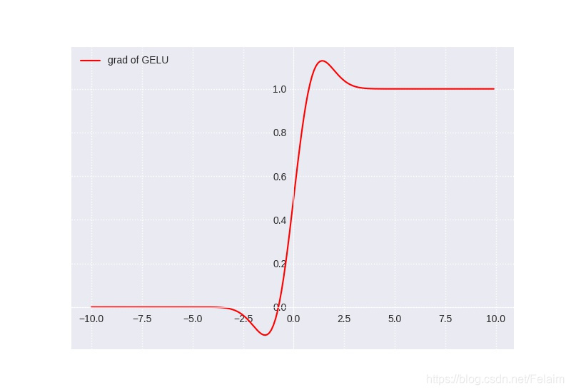
6. GELU

公式：

$\text{GELU}(x)=x\ast \Phi (x)$

$\Phi (x)$ is the Cumulative Distribution Function for Gaussian Distribution

GELU的函数形状如下图所示:

对应的导数形式如下图所示：

GELU函数的优点：

• 之前描述的所有的激活函数正则化和激活函数是分开进行的，GELU是同时进行正则化和激活函数

GELU函数的缺点：

• 暂无，等待补充

PS： 上述图例代码

import torch
import matplotlib.pylab as plt
import torch.nn.functional as F
import osfunc_pic_res = "./func_pic_res/"
if not os.path.exists(func_pic_res):os.makedirs(func_pic_res)def xyplot(x_vals, y_vals, name):plt.figure()plt.rcParams['figure.figsize'] = (5, 3.5)plt.plot(x_vals.detach().numpy(), y_vals.detach().numpy(), label=name, linewidth=1.5, color='#FF0000')plt.grid(True, linestyle=':')plt.legend(loc='upper left')# dark_background, seaborn, ggplotplt.style.use("seaborn")ax = plt.gca()ax.spines['right'].set_color("none")ax.spines['top'].set_color("none")ax.spines['bottom'].set_position(("data", 0))ax.spines['left'].set_position(("data", 0))ax.spines['bottom'].set_linewidth(0.5)ax.spines['left'].set_linewidth(0.5)ax.xaxis.set_ticks_position('bottom')ax.yaxis.set_ticks_position('left')plt.savefig(func_pic_res + "{}.jpg".format(name))# sigmoid激活函数
def test_Sigmoid():x = torch.arange(-10.0, 10.0, 0.1, requires_grad=True)y = x.sigmoid()xyplot(x, y, 'Sigmoid')# 导数y.sum().backward()xyplot(x, x.grad, 'grad of Sigmoid')def test_Tanh():x = torch.arange(-10.0, 10.0, 0.1, requires_grad=True)y = x.tanh()xyplot(x, y, 'Tanh')# 导数y.sum().backward()xyplot(x, x.grad, 'grad of Tanh')def test_ReLU():x = torch.arange(-10.0, 10.0, 0.1, requires_grad=True)y = x.relu()xyplot(x, y, 'ReLU')# 导数y.sum().backward()xyplot(x, x.grad, 'grad of ReLU')def test_LeakyReLU():x = torch.arange(-10.0, 10.0, 0.1, requires_grad=True)y = F.leaky_relu(x, negative_slope=0.1, inplace=False)xyplot(x, y, 'LeakyReLU(negative_slope=0.1)')# 导数y.sum().backward()xyplot(x, x.grad, 'grad of LeakyReLU(negative_slope=0.1)')def test_ELU():x = torch.arange(-10.0, 10.0, 0.1, requires_grad=True)y = F.elu(x, alpha=0.3, inplace=False)xyplot(x, y, 'ELU(alpha=0.3)')# 导数y.sum().backward()xyplot(x, x.grad, 'grad of ELU(alpha=0.3)')def test_GELU():x = torch.arange(-10.0, 10.0, 0.1, requires_grad=True)y = F.gelu(x)xyplot(x, y, 'GELU')# 导数y.sum().backward()xyplot(x, x.grad, 'grad of GELU')if __name__ == "__main__":test_Sigmoid()test_Tanh()test_ReLU()test_LeakyReLU()test_ELU()test_GELU()