文章目录
- 回声状态网络
- 状态方程
- 输出方程
- 分类问题
- 加载 MNIST 数据集
- 标签 onehot 编码
- 转化成时间序列
- 训练 ESN
- 储备池状态的时空分布
- 测试结果

回声状态网络
状态方程

输出方程

分类问题

加载 MNIST 数据集
from torchvision.datasets import mnist train_set = mnist.MNIST('./data', train=True, download=True)    # 若未找到数据集 则自动下载
test_set = mnist.MNIST('./data', train=False, download=True)print(train_set.data.shape,  train_set.targets.shape)
"""
(torch.Size([60000, 28, 28]), torch.Size([60000]))
"""
同时也下载到了本地

标签 onehot 编码
data = train_set.data.numpy()
labels = train_set.targets.numpy().reshape(-1,1)
enc = OneHotEncoder()
enc.fit(labels)
labels_onehot = enc.transform(labels).toarray()
"""
>>> labels_onehot
array([[0., 0., 0., ..., 0., 0., 0.],[1., 0., 0., ..., 0., 0., 0.],[0., 0., 0., ..., 0., 0., 0.],...,[0., 0., 0., ..., 0., 0., 0.],[0., 0., 0., ..., 0., 0., 0.],[0., 0., 0., ..., 0., 1., 0.]])
"""
转化成时间序列
num_train = 1000
# input
U = np.hstack(data[:num_train])/255
# output
y = np.hstack([np.array([labels_onehot[i] for _ in range(28)]).T for i in range(num_train)])
图像是28 * 28 的,通过拼接,作为输入的 28 维时间序列

预测标签为 10 维时间序列序列,长度和输入相同

训练 ESN
设置随机种子
import numpy as np
import matplotlib.pyplot as plt
import scipy.linalg
import randomdef set_seed(seed=None):"""Making the seed (for random values) variable if None"""# Set the seedif seed is None:import timeseed = int((time.time()*10**6) % 10**12)try:random.seed(seed) #np.random.seed(seed)print("Seed used for random values:", seed)except:print("!!! WARNING !!!: Seed was not set correctly.")return seed
开始训练
T = y.shape[1]
# generate the ESN reservoir
inSize = 28
outSize = 10 #input/output dimension
resSize = 1000 #reservoir size
a = 0.8 # leaking rate
spectral_radius = 1.25
reg = 1e-8 # regularization coefficient
input_scaling = 1.# change the seed, reservoir performances should be averaged accross at least 20 random instances (with the same set of parameters)
our_seed = None  # Choose a seed or None
set_seed(our_seed) # generation of random weights
Win = (np.random.rand(resSize,1+inSize)-0.5) * input_scaling
W = np.random.rand(resSize,resSize)-0.5# Computing spectral radius...
rhoW = max(abs(np.linalg.eig(W)[0])) #maximal eigenvalue
W *= spectral_radius / rhoWX = np.zeros((1+inSize+resSize,T))# set the corresponding target matrix directly
Yt = y # run the reservoir with the data and collect X
x = np.zeros((resSize,1))  # initial state
for t in range(U.shape[1]):u = U[:,t:t+1]res_in = np.dot( Win, np.vstack((1,u))) + np.dot( W, x )res_out = sigmoid(res_in)x = (1-a) * x + a * res_out X[:,t] = np.vstack((1,u,x))[:,0]X_T = X.T
# use ridge regression (linear regression with regularization)
Wout = np.dot( np.dot(Yt,X_T), np.linalg.inv( np.dot(X,X_T) + reg*np.eye(1+inSize+resSize)))
import seaborn as sns
plt.figure(figsize=(20,10))
ax = sns.heatmap(X)
plt.show()
print('done')
储备池状态的时空分布
看看训练储备池状态的时空分布,下图展示前10个数字对应的 X, 第 1~28 行是原始输入,和储备池的 1000 维状态向量拼接在一起
可以观察到出现数字时,储备池的状态会有明显变化

测试结果
test_start = 50000
num_test = 10
U = np.hstack(data[test_start:test_start + num_test])/255
y = np.hstack([np.array([labels_onehot[i] for _ in range(28)]).T for i in range(test_start,test_start + num_test)])
输入:

真实标签:

输出结果:
T = y.shape[1]
# allocated memory for the design (collected states) matrix
X = np.zeros((1+inSize+resSize,T))x = np.zeros((resSize,1))
for t in range(U.shape[1]):u = U[:,t:t+1]res_in = np.dot( Win, np.vstack((1,u))) + np.dot( W, x )res_out = sigmoid(res_in)x = (1-a) * x + a * res_out       X[:,t] = np.vstack((1,u,x))[:,0]pred = Wout @ X
plt.figure(figsize=(20,5))
sns.heatmap(np.vstack([pred,y]))
plt.show()

结果中 10 个对了 9 个,其中预测错误的第七个样本把 5 判别成 8