Python代码实现了fft与逆fft。
参考资料:
https://walkccc.github.io/CLRS/Chap30/30.1/
https://sites.math.rutgers.edu/~ajl213/CLRS/Ch30.pdf

30 Polynomials and the FFT

30.1 Representing polynomials

1.Multiply the polynomials $A(x) = 7x^3 - x^2 + x - 10$ and $B(x) = 8x^3 - 6x + 3$ using equations (30.1) and (30.2).

$\begin{array}{rl} & 56x^6 - 8x^5 + (8 - 42)x^4 + (-80 + 6 + 21)x^3 + (-3 - 6)x^2 + (60 + 3)x - 30 \\ = & 56x^6 - 8x^5 - 34x^4 - 53x^3 - 9x^2 + 63x - 30. \end{array}$

2.Another way to evaluate a polynomial A(x) of degree-bound n at a given point $x_0$ is to divide A(x) by the polynomial $(x - x_0)$ , obtaining a quotient polynomial q(x) of degree-bound n - 1 and a remainder r, such that

$A(x) = q(x)(x - x_0) + r$

Clearly, $A(x_0) = r$ . Show how to compute the remainder r and the coefficients of q(x) in time $\Theta(n)$ from $x_0$ and the coefficients of A.

Let A be the matrix with 1's on the diagonal, $−x_0$ $-x_0$ 's on the super diagonal, and 0's everywhere else. Let q be the vector $(r, q_0, q_1, \dots, x_{n-2})$ . If $a = (a_0, a_1, \dots, a_{n-1})$ then we need to solve the matrix equation Aq = a to compute the remainder and coefficients. Since A is tridiagonal, Problem 28-1 (e) tells us how to solve this equation in linear time.

3.Derive a point-value representation for $A^\text{rev}(x) = \sum_{j = 0}^{n - 1} a_{n - 1 - j}x^j$ from a point-value representation for $A(x) = \sum_{j = 0}^{n - 1} a_jx^j$ , assuming that none of the points is 0.

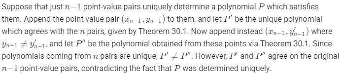
4.Prove that n distinct point-value pairs are necessary to uniquely specify a polynomial of degree-bound nn, that is, if fewer than nn distinct point-value pairs are given, they fail to specify a unique polynomial of degree-bound n. Hint: Using Theorem 30.1, what can you say about a set of n - 1 point-value pairs to which you add one more arbitrarily chosen point-value pair?)

5.Show how to use equation (30.5) to interpolate in time $\Theta(n^2)$ . Hint: First compute the coefficient representation of the polynomial $\prod_j (x - x_j)$ and then divide by $(x - x_k)$ as necessary for the numerator of each term; see Exercise 30.1-2. You can compute each of the nn denominators in time O(n).

6.Explain what is wrong with the "obvious" approach to polynomial division using a point-value representation, i.e., dividing the corresponding yy values. Discuss separately the case in which the division comes out exactly and the case in which it doesn't.

If we wish to compute P/Q but Q takes on the value zero at some of these points, then we can't carry out the "obvious" method. However, as long as all point value pairs $(x_i, y_i)$ we choose for Q are such that $y_i \ne 0$ , then the approach comes out exactly as we would like.

7.Consider two sets A and B, each having n integers in the range from 0 to 10n. We wish to compute the Cartesian sum of A and B, defined by

$C = \{x + y: x \in A \text{ and } y \in B\}$

Note that the integers in C are in the range from 0 to 20n. We want to find the elements of C and the number of times each element of C is realized as a sum of elements in A and B. Show how to solve the problem in O(nlgn) time.Hint: Represent A and B as polynomials of degree at most 10n.

30.2 The DFT and FFT

1.Prove Corollary 30.4.

根据引理30.3消去引理，这里设d=n/2，k=2，就可以得出：

$w_n^{n/2}=w_2=-1$

2.Compute the DFT of the vector (0,1,2,3).

$y_0 = 0*w_4^0 + 1*w_4^{0*1} + 2*w_4^{0*2} + 3*w_4^{0*3} = 0 + 1+ 2+3 =6$

$y_1 = 0*w_4^{1*0} + 1*w_4^{1*1} + 2*w_4^{1*2} + 3*w_4^{1*3}=i-2-3i = -2-2i$

$y_2 = 0*w_4^{2*0} + 1*w_4^{2*1} + 2*w_4^{2*2} + 3*w_4^{2*3}= -1 + 2 -3 =-2$

$y_3 = 0*w_4^{3*0} + 1*w_4^{3*1} + 2*w_4^{3*2} + 3*w_4^{3*3}= -i - 2 +3i =2i-2$

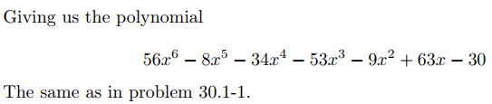
3.Do Exercise 30.1-1 by using the Θ(nlgn)-time scheme.

4.Write pseudocode to compute $\text{DFT}_n^{-1}$ Θ(nlgn) time.

Python代码：

1).DFT:

import numpy as npdef recursive_fft(a):n = len(a)if n == 1:return aw_n = np.exp(complex(0,2*np.pi/n))w = 1a0 = a[0:n:2]a1 = a[1:n:2]y0 = recursive_fft(a0)y1 = recursive_fft(a1)y = np.zeros(n,dtype='complex')for k in np.arange(0,n//2):y[k] = y0[k] + w*y1[k]y[k + n//2] = y0[k] - w*y1[k]w = w*w_nreturn yprint(recursive_fft([0,1,2,3]))

示例计算了本节习题2，输出为：[ 6.+0.j -2.-2.j -2.+0.j -2.+2.j]

2).逆DFT：

import numpy as npdef recursive_inverse_fft_base(y):n = len(y)if n == 1:return yw_n = np.exp(complex(0,-2*np.pi/n))w = 1y0 = y[0:n:2]y1 = y[1:n:2]a0 = recursive_inverse_fft_base(y0)a1 = recursive_inverse_fft_base(y1)a = np.zeros(n,dtype='complex')for k in np.arange(0,n//2):a[k] = (a0[k] + w*a1[k])a[k + n//2] = (a0[k] - w*a1[k])w = w*w_nreturn adef recursive_inverse_fft(y):a = recursive_inverse_fft_base(y)return a / len(y)print(recursive_inverse_fft([6,-2-2j,-2,-2+2j]))

这是对本节第2题求逆，结果应该是[0,1,2,3].代码运行结果为：

[0.+0.000000e+00j 1.-6.123234e-17j 2.+0.000000e+00j 3.+6.123234e-17j]

第2项和第4项有一个极小的j，这是计算浮点数的误差导致，可以认为是0，结果就是[0,1,2,3].

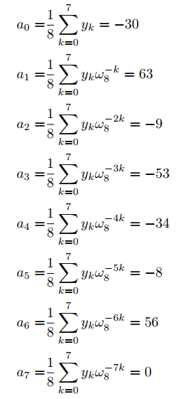
3).结合fft的代码计算本节第3题：

a = np.array([7,-1,1,-10,0,0,0,0])
b = np.array([8,0,-6,3,0,0,0,0])
ya = recursive_fft(a)
yb = recursive_fft(b)
yc = ya*yb
c = recursive_inverse_fft(yc)
print(c)

输出结果：

[ 56.-3.55271368e-15j -8.+8.75870054e-15j -34.+0.00000000e+00j
-53.-6.98234370e-15j -9.+3.55271368e-15j 63.-5.45215418e-15j
-30.+0.00000000e+00j 0.+3.67579734e-15j]

因为我们做了后补0，因此需要把输出中最后一项0去掉，系数从高到低就是[56,-8,-34,-53,-9,63,-30]

5.Describe the generalization of theFFT procedure to the case in which nn is a power of 3. Give a recurrence for the running time, and solve the recurrence.

6.Suppose that instead of performing an nn-element FFT over the field of complex numbers (where nn is even), we use the ring Zm of integers modulo m, where $m = 2^{tn / 2} + 1$ and t is an arbitrary positive integer. Use $\omega = 2^t$ instead of $\omega_n$ as a principal nth root of unity, modulo mm. Prove that the DFT and the inverse DFT are well defined in this system.

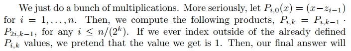
7.Given a list of values $z_0, z_1, \dots, z_{n - 1}$ (possibly with repetitions), show how to find the coefficients of a polynomial P(x) of degree-bound n+1 that has zeros only at $z_0, z_1, \dots, z_{n - 1}$ (possibly with repetitions). Your procedure should run in time $O(n\lg^2 n)$ . (Hint: The polynomial P(x) has a zero at $z_j$ if and only if P(x) is a multiple of $(x - z_j)$

8.The chirp transform of a vector $a = (a_0, a_1, \dots, a_{n - 1})$ is the vector $y = (y_0, y_1, \dots, y_{n - 1})$ , where $y_k = \sum_{j = 0}^{n - 1} a_jz^{kj}$ and z is any complex number. The DFT is therefore a special case of the chirp transform, obtained by taking $z = \omega_n$ . Show how to evaluate the chirp transform in time $O(n\lg n)$ for any complex number z. Hint: Use the equation

$y_k = z^{k^2 / 2} \sum_{j = 0}^{n - 1} \Big(a_jz^{j^2 / 2}\Big) \Big(z^{-(k - j)^2 / 2}\Big)$

to view the chirp transform as a convolution.)

30.3 Efficient FFT implementations

1.Show how ITERATIVE-FFT computes the DFT of the input vector (0,2,3,−1,4,5,7,9).

2.Show how to implement an FFT algorithm with the bit-reversal permutation occurring at the end, rather than at the beginning, of the computation. Hint: Consider the inverse DFT.

We can consider ITERATIVE-FFT as working in two steps, the copy step (line 1) and the iteration step (lines 4 through 14). To implement in inverse
iterative FFT algorithm, we would need to first reverse the iteration step, then reverse the copy step. We can do this by implementing the INVERSEINTERATIVE-FFT algorithm exactly as we did with the FFT algorithm, but this time creating the iterative version of RECURSIVE-FFT-INV as given in exercise 30.2-4.

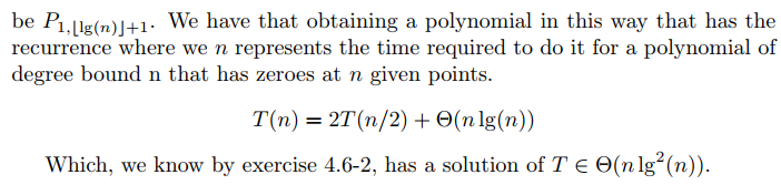
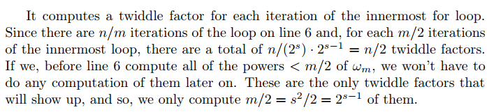
3.How many times does ITERATIVE-FFT compute twiddle factors in each stage? Rewrite ITERATIVE-FFT to compute twiddle factors only $2^{s - 1}$ times in stage s.

4.Suppose that the adders within the butterfly operations of the FFT circuit sometimes fail in such a manner that they always produce a zero output, independent of their inputs. Suppose that exactly one adder has failed, but that you don't know which one. Describe how you can identify the failed adder by supplying inputs to the overall FFT circuit and observing the outputs. How efficient is your method?

First observe that if the input to a butterfly operation is all zeros, then so is the output. Our initial input will be ( $a_0,a_1...a_{n-1}$ ) where $a_i = 0$ if 0 ≤ i ≤ n/2 - 1, and i otherwise. By examining the diagram on page 919, we see that the zeros will propogate as half the input to each butterfly operation in the final stage. Thus, if any of the output values are 0 we know that one of
the $y_k$ ’s is zero, where k ≥ n/2 - 1. If this is the case, then the faulty butterfly added occurs along the wire connected to yk. If none of the output values are zero, the faulty butterfly adder must occur as one which only deals with the first n/2 - 1 wires. In this case, we rerun the test with input such that $a_i = i$ if 0 ≤ i ≤ n=2 - 1 and 0 otherwise. This time, we will know for sure which of the first n/2-1 wires touches the faulty butterfly adder. Since only lg n adders touch a given wire, we have reduced the problem of size n to a problem of size lg n. Thus, at most $2 lg^* n = O(lg^*n)$ tests are required.

Problems

1.Divide-and-conquer multiplication:

a. Show how to multiply two linear polynomials ax + b and cx + d using only three multiplications. Hint: One of the multiplications is $(a + b) \cdot (c + d)$

b. Give two divide-and-conquer algorithms for multiplying two polynomials of degree-bound nn inΘ(nlg3) time. The first algorithm should divide the input polynomial coefficients into a high half and a low half, and the second algorithm should divide them according to whether their index is odd or even.

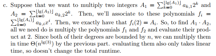
c. Show how to multiply two nn-bit integers in O(nlg3) steps, where each step operates on at most a constant number of 1-bit values.

2.A Toeplitz matrix is an n×n matrix $A = (a_{ij})$ such that $a_{ij} = a_{i - 1, j - 1}$ for $i = 2, 3, \dots, n$ and $j = 2, 3, \dots, n$ .

a. Is the sum of two Toeplitz matrices necessarily Toeplitz? What about the product?

b. Describe how to represent a Toeplitz matrix so that you can add two n×n Toeplitz matrices in O(n) time.

c. Give an O(nlgn)-time algorithm for multiplying an n×n Toeplitz matrix by a vector of length n. Use your representation from part (b).

d. Give an efficient algorithm for multiplying two n×n Toeplitz matrices. Analyze its running time.

3. Multidimensional fast Fourier transform

We can generalize the 1-dimensional discrete Fourier transform defined by equation(30.8) to d dimensions. The input is a d-dimensional array $A = (a_{j_1, j_2, \dots, j_d})$ whose dimensions are $n_1, n_2, \dots, n_d$ , where $n_1n_2 \cdots n_d = n$ . We define the d-dimensional discrete Fourier transform by the equation

$y_{k_1, k_2, \dots, k_d} = \sum_{j_1 = 0}^{n_1 - 1} \sum_{j_2 = 0}^{n_2 - 1} \cdots \sum_{j_d = 0}^{n_d - 1} a_{j_1, j_2, \cdots, j_d} \omega_{n_1}^{j_1k_1}\omega_{n_2}^{j_2k_2} \cdots \omega_{n_d}^{j_dk_d}$

for $0 \le k_1 < n_1, 0 \le k_2 < n_2, \dots, 0 \le k_d < n_d$

a. Show that we can compute a dd-dimensional DFT by computing 1-dimensional DFTs on each dimension in turn. That is, we first compute $n/n_1$ separate 1-dimensional DFTs along dimension 1. Then, using the result of the DFTs along dimension 1 as the input, we compute $n/n_2$ separate 1-dimensional DFTs along dimension 2. Using this result as the input, we compute $n / n_3$ separate 1-dimensional DFTs along dimension 3, and so on, through dimension d.

b. Show that the ordering of dimensions does not matter, so that we can compute a d-dimensional DFT by computing the 1-dimensional DFTs in any order of the d dimensions.

c. Show that if we compute each 1-dimensional DFT by computing the fast Fourier transform, the total time to compute a d-dimensional DFT is O(nlgn), independent of d.

4.Evaluating all derivatives of a polynomial at a point

Given a polynomial A(x) of degree-bound n, we define its tth derivative by

$A^{(t)}(x) = \begin{cases} A(x) & \text{ if } t = 0, \\ \frac{d}{dx} A^{(t - 1)}(x) & \text{ if } 1 \le t \le n - 1, \\ 0 & \text{ if } t \ge n. \end{cases}$

From the coefficient representation $(a_0, a_1, \dots, a_{n - 1})$ of A(x) and a given point $x_0$ , we wish to determine $A^{(t)}(x_0)$ for $t = 0, 1, \dots, n- 1$ .

a. Given coefficients $b_0, b_1, \dots, b_{n - 1}$ such that

$A(x) = \sum_{j = 0}^{n - 1} b_j(x - x_0)^j$

show how to compute $A^{(t)}(x_0)$ for $t = 0, 1, \dots, n - 1$ in O(n) time.

b. Explain how to find $b_0, b_1, \dots, b_{n - 1}$ in $O(n\lg n)$ time, given $A(x_0 + \omega_n^k)$ for $k = 0, 1, \dots, n - 1$ .

c. Prove that

$A(x_0 + \omega_n^k) = \sum_{r = 0}^{n - 1} \Bigg(\frac{\omega_n^{kr}}{r!} \sum_{j = 0}^{n - 1} f(j)g(r - j)\Bigg)$

where $f(j) = a_j \cdot j!$ and

$g(l) = \begin{cases} x_0^{-l} / (-l)! & \text{ if } -(n - 1) \le l \le 0, \\ 0 & \text{ if } 1 \le l \le n - 1. \end{cases}$

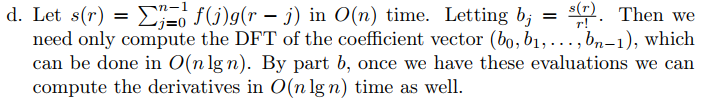
d. Explain how to evaluate $A(x_0 + \omega_n^k)$ for $k = 0, 1, \dots, n - 1$ in O(nlgn) time. Conclude that we can evaluate all nontrivial derivatives of A(x) at $x_0$ in O(nlgn) time.

5. Polynomial evaluation at multiple points

We have seen how to evaluate a polynomial of degree-bound nn at a single point in O(n) time using Horner's rule. We have also discovered how to evaluate such a polynomial at all n complex roots of unity in O(nlgn) time using the FFT. We shall now show how to evaluate a polynomial of degree-bound n at n arbitrary points in $O(n\lg^2 n)$ time.

To do so, we shall assume that we can compute the polynomial remainder when one such polynomial is divided by another inO(nlgn) time, a result that we state without proof. For example, the remainder of $3x^3 + x^2 - 3x + 1$ when divided by $x^2 + x + 2$ is

$(3x^3 + x^2 - 3x + 1) \mod (x^2 + x + 2) = -7x + 5$ .

Given the coefficient representation of a polynomial $A(x) = \sum_{k = 0}^{n - 1} a_kx^k$ and n points $x_0, x_1, \dots, x_{n - 1}$ , we wish to compute the n values $A(x_0), A(x_1), \dots, A(x_{n - 1})$ . For $0 \le i \le j \le n - 1$ , define the polynomials $P_{ij}(x) = \prod_{k = i}^j (x - x_k)$ and $Q_{ij}(x) = A(x) \mod P_{ij}(x)$ . Note that $Q_{ij}(x)$ has degree at most j - i.

a. Prove that $A(x) \mod (x - z) = A(z)$ for any point zz.

b. Prove that $Q_{kk}(x) = A(x_k)$ and that $Q_{0, n - 1}(x) = A(x)$ .

c. Prove that for $i \le k \le j$ , we have $Q_{ik}(x) = Q_{ij}(x) \mod P_{ik}(x)$ and $Q_{kj}(x) = Q_{ij}(x) \mod P_{kj}(x)$

d. Give an $O(n\lg^2 n)$ -time algorithm to evaluate $A(x_0), A(x_1), \dots, A(x_{n - 1})$

6. FFT using modular arithmetic

As defined, the discrete Fourier transform requires us to compute with complex numbers, which can result in a loss of precision due to round-off errors. For some problems, the answer is known to contain only integers, and by using a variant of the FFT based on modular arithmetic, we can guarantee that the answer is calculated exactly. An example of such a problem is that of multiplying two polynomials with integer coefficients. Exercise 30.2-6 gives one approach, using a modulus of length Ω(n) bits to handle a DFT on n points. This problem gives another approach, which uses a modulus of the more reasonable lengthO(lgn); it requires that you understand the material of Chapter 31. Let n be a power of 2.

a. Suppose that we search for the smallest k such thatp=kn+1 is prime. Give a simple heuristic argument why we might expect k to be approximately lnn. (The value of k might be much larger or smaller, but we can reasonably expect to examineO(lgn) candidate values of k on average.) How does the expected length of pp compare to the length of n?

Let g be a generator of $\mathbb Z_p^*$ , and let $w = g^k \mod p$ .

b. Argue that the DFT and the inverseDFT are well-defined inverse operations modulo p, where w is used as a principal nth root of unity.

c. Show how to make the FFT and its inverse work modulo p in time O(nlgn), where operations on words of O(lgn) bits take unit time. Assume that the algorithm is given p and w.

d. Compute the DFT modulo p=17 of the vector (0,5,3,7,7,2,1,6). Note that g=3 is a generator of $\mathbb Z_{17}^*$ .