参考文献:
https://walkccc.me/CLRS/Chap29/29.1/
https://sites.math.rutgers.edu/~ajl213/CLRS/
29.Linear Programming
29.1 Standard and slack forms
1.If we express the linear program in (29.24)–(29.28) in the compact notation of (29.19)–(29.21), what are n, m, A, b, and c?
2.Give three feasible solutions to the linear program in (29.24)–(29.28). What is the objective value of each one?
with objective value 9.
with objective value 4.
with objective value −1.
3.For the slack form in (29.38)–(29.41), what are N, B, A, b, c, and v?
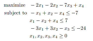
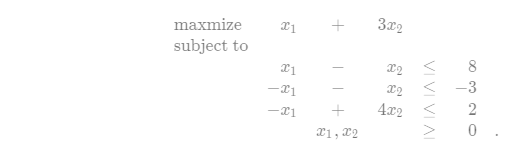
4.Convert the following linear program into standard form:
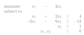
5.Convert the following linear program into slack form:
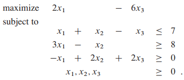
What are the basic and nonbasic variables?
First, we will multiply the second and third inequalities by minus one to make it so that they are all inequalities. We will introduce the three new variables
, and perform the usual procedure for rewriting in slack form
where we are still trying to maximize . The basic variables are
and the nonbasic variables are
.
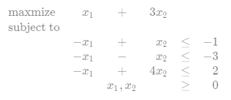
6.Show that the following linear program is infeasible:
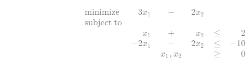
By dividing the second constraint by 2 and adding to the first, we have 0≤−3, which is impossible. Therefore there linear program is unfeasible.
7.Show that the following linear program is unbounded:

8.Suppose that we have a general linear program with n variables and m constraints, and suppose that we convert it into standard form. Give an upper bound on the number of variables and constraints in the resulting linear program.
In the worst case, we have to introduce 2 variables for every variable to ensure that we have nonnegativity constraints, so the resulting program will have 2n variables. If each constraint is an equality, we would have to double the number of constraints to create inequalities, resulting in 2m constraints. Changing minimization to maximization and greater-than signs to less-than signs don't affect the number of variables or constraints, so the upper bound is 2n on variables and 2m on constraints.
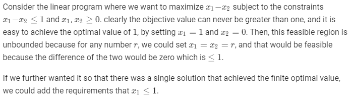
9.Give an example of a linear program for which the feasible region is not bounded, but the optimal objective value is finite.
29.2 Formulating problems as linear programs
1.Put the single-pair shortest-path linear program from (29.44)–(29.46) into standard form.
The objective is already in normal form. However, some of the constraints are equality constraints instead of ≤ constraints. This means that we need to rewrite them as a pair of inequality constraints, the overlap of whose solutions is just the case where we have equality. we also need to deal with the fact that most of the variables can be negative. To do that, we will introduce variables for the negative part and positive part, each of which need be positive, and we'll just be sure to subtract the negative part. d_sds need not be changed in this way since it can never be negative since we are not assuming the existence of negative weight cycles.
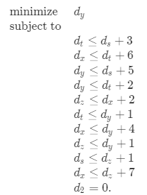
2.Write out explicitly the linear program corresponding to finding the shortest path from node ss to node y in Figure 24.2(a).
3.In the single-source shortest-paths problem, we want to find the shortest-path weights from a source vertex s to all vertices v∈V. Given a graph G, write a linear program for which the solution has the property that is the shortest-path weight from s to v for each vertex
.
We will follow a similar idea to the way to when we were finding the shortest path between two particular vertices.
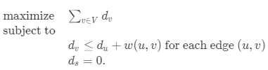
The first type of constraint makes sure that we never say that a vertex is further away than it would be if we just took the edge corresponding to that constraint. Also, since we are trying to maximize all of the variables, we will make it so that there is no slack anywhere, and so all the values will correspond to lengths of shortest paths to v. This is because the only thing holding back the variables is the information about relaxing along the edges, which is what determines shortest paths.
4.Write out explicitly the linear program corresponding to finding the maximum flow in Figure 26.1(a).

5.Rewrite the linear program for maximum flow (29.47)–(29.50) so that it uses only O(V+E) constraints.

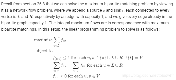
6.Write a linear program that, given a bipartite graph G = (V, E) solves the maximum-bipartite-matching problem.
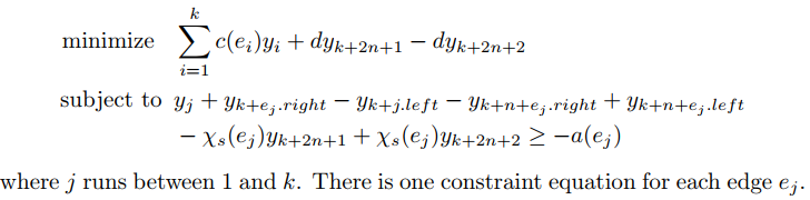
7.In the minimum-cost multicommodity-flow problem, we are given directed graph G=(V,E) in which each edge (u,v)∈E has a nonnegative capacityc(u,v)≥0 and a costa(u,v). As in the multicommodity-flow problem, we are given k different commodities, , where we specify commodity ii by the triple
. We define the flow
for commodity i and the aggregate flow
on edge (u,v) as in the multicommodity-flow problem. A feasible flow is one in which the aggregate flow on each edge (u,v) is no more than the capacity of edge (u,v). The cost of a flow is
, and the goal is to find the feasible flow of minimum cost. Express this problem as a linear program.


29.3 The simplex algorithm
1.Complete the proof of Lemma 29.4 by showing that it must be the case that c = c' and v = v' .

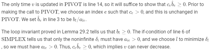
2.Show that the call to PIVOT in line 12 of SIMPLEX never decreases the value of v.
3.Prove that the slack form given to the PIVOT procedure and the slack form that the procedure returns are equivalent.
To show that the two slack forms are equivalent, we will show both that they have equal objective functions, and their sets of feasible solutions are equal.
First, we'll check that their sets of feasible solutions are equal. Basically all we do to the constraints when we pivot is take the non-basic variable, e, and solve the equation corresponding to the basic variable l for e. We are then taking that expression and replacing e in all the constraints with this expression we got by solving the equation corresponding to l. Since each of these algebraic operations are valid, the result of the sequence of them is also algebraically equivalent to the original.
Next, we'll see that the objective functions are equal. We decrease each by
, which is to say that we replace the non-basic variable we are making basic with the expression we got it was equal to once we made it basic.
Since the slack form returned by PIVOT, has the same feasible region and an equal objective function, it is equivalent to the original slack form passed in.
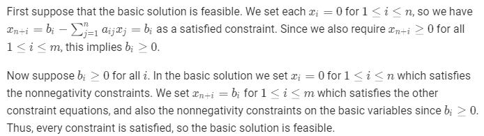
4.Suppose we convert a linear program (A, b, c) in standard form to slack form. Show that the basic solution is feasible if and only if for
.
5.Solve the following linear program using SIMPLEX:
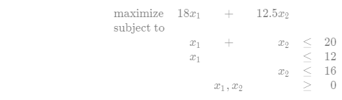

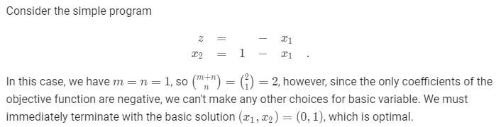
6.Solve the following linear program using SIMPLEX:

very nonbasic variable now has negative coefficient in the objective function, so we take the basic solution . The objective value this achieves is 5.
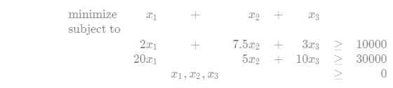
7.Solve the following linear program using SIMPLEX:


8.In the proof of Lemma 29.5, we argued that there are at most ways to choose a set B of basic variables. Give an example of a linear program in which there are strictly fewer than
ways to choose the set B.
29.4 Duality
1.Formulate the dual of the linear program given in Exercise 29.3-5.
By just transposing A, swapping b and c, and switching the maximization to a minimization, we want to minimize subject to the constrain
2.Suppose that we have a linear program that is not in standard form. We could produce the dual by first converting it to standard form, and then taking the dual. It would be more convenient, however, to be able to produce the dual directly. Explain how we can directly take the dual of an arbitrary linear program.
By working through each aspect of putting a general linear program into standard form, as outlined on page 852, we can show how to deal with transforming each into the dual individually. If the problem is a minimization instead of a maximization, replace by
in (29.84). If there is a lack of nonnegativity constraint on
we duplicate the jth column of A, which corresponds to duplicating the jth row of
. If there is an equality constraint for
, we convert it to two inequalities by duplicating then negating the iith column of
, duplicating then negating the ith entry of b, and adding an extra
variable. We handle the greater-than-or-equal-to sign
by negating iith column of
and negating
. Then we solve the dual problem of minimizing
subject to
and y≥0.
3.Write down the dual of the maximum-flow linear program, as given in lines (29.47)–(29.50) on page 860. Explain how to interpret this formulation as a minimum-cut problem.


4.Write down the dual of the minimum-cost-flow linear program, as given in lines(29.51)(29.52) on page 862. Explain how to interpret this problem in terms of graphs and flows.

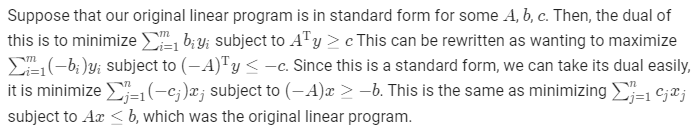
5.Show that the dual of the dual of a linear program is the primal linear program.
6.Which result from Chapter 26 can be interpreted as weak duality for the maximum-flow problem?
Corollary 26.5 from Chapter 26 can be interpreted as weak duality.
29.5 The initial basic feasible solution
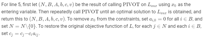
1.Give detailed pseudocode to implement lines 5 and 14 of INITIALIZE-SIMPLEX.
2.Show that when the main loop of SIMPLEX is run by INITIALIZE-SIMPLEX, it can never return "unbounded."
In order to enter line 10 of INITIALIZE-SIMPLEX and begin iterating the main loop of SIMPLEX, we must have recovered a basic solution which is feasible for. Since
and the objective function is
, the objective value associated to this solution (or any solution) must be negative. Since the goal is to aximize, we have an upper bound of 0 on the objective value. By Lemma 29.2,SIMPLEX correctly determines whether or not the input linear program is unbounded. Since
is not unbounded, this can never be returned by SIMPLEX.
3.Suppose that we are given a linear program L in standard form, and suppose that for both L and the dual of L, the basic solutions associated with the initial slack forms are feasible. Show that the optimal objective value of L is =0.
Since it is in standard form, the objective function has no constant term, it is entirely given by , which is going to be zero for any basic solution. The same thing goes for its dual. Since there is some solution which has the objective function achieve the same value both for the dual and the primal, by the corollary to the weak duality theorem, that common value must be the optimal value of the objective function.
4.Suppose that we allow strict inequalities in a linear program. Show that in this case, the fundamental theorem of linear programming does not hold.
Consider the linear program in which we wish to maximize subject to the constraint
and
. This has no optimal solution, but it is clearly bounded and has feasible solutions. Thus, the Fundamental theorem of linear programming does not hold in the case of strict inequalities.
5.Solve the following linear program using SIMPLEX:


6.Solve the following linear program using SIMPLEX:


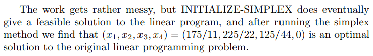
7.Solve the following linear program using SIMPLEX:


8.Solve the linear program given in (29.6)–(29.10).


9.Consider the following 1-variable linear program, which we call P:

- One option is that r = 0,s≥0 and t≤0. Suppose that r>0, then, if we have that s is non-negative and tt is non-positive, it will be as we want.
- We will split into two cases based on r. If r = 0, then this is exactly when tt is non-positive and s is non-negative. The other possible case is that r is negative, and t is positive. In which case, because r is negative, we can always get rx as small as we want so s doesn't matter, however, we can never make rx positive so it can never be ≥t.
- Again, we split into two possible cases for r. If r=0, then it is when t is nonnegative and s is non-positive. The other possible case is that r is positive, and s is negative. Since r is positive, rx will always be non-negative, so it cannot be ≤s. But since r is positive, we have that we can always make rx as big as we want, in particular, greater than tt.
- If we have that r=0 and t is positive and s is negative. If r is nonzero, then we can always either make rx really big or really small depending on the sign of r, meaning that either the primal or the dual would be feasable.
Problems
1.Linear-inequality feasibility


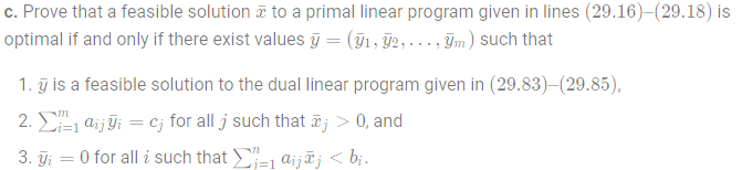
2.Complementary slackness


3.Integer linear programming


4.Farkas'ss lemma


5.Minimum-cost circulation