Python实现预测信用卡潜在客户

一、数据集

有一家名为Happy Customer Bank (快乐客户银行) 的银行，是一家中型私人银行，经营各类银行产品，如储蓄账户、往来账户、投资产品、信贷产品等。

该银行还向现有客户交叉销售产品，为此他们使用不同类型的通信方式，如电话、电子邮件、网上银行推荐、手机银行等。

在这种情况下，Happy Customer Bank 希望向现有客户交叉销售其信用卡。该银行已经确定了一组有资格使用这些信用卡的客户。

银行希望确定对推荐的信用卡表现出更高意向的客户。

数据集：dataset

该数据集主要包括：

客户详细信息（gender, age, region, etc）
他/她与银行的关系详情（Channel_Code、Vintage、Avg_Asset_Value, etc）

在这里，我们的任务是构建一个能够识别对信用卡感兴趣的客户的模型。

二、本文实现的模型

完成了LR、RF、LIGHTBGM、XGBOOST等模型的预测

三、代码

import numpy as np
import pandas as pd
import matplotlib.pyplot as plt
import seaborn as sns
import warnings
warnings.filterwarnings('ignore')
# Import dataset
df_train = pd.read_csv(r"C:\Users\Administrator\Desktop\DATA\Credit-Card-Lead-Prediction-main\train_s3TEQDk.csv")
df_train.head()
# Shape of the data
df_train.shape# There is 2.45L rows and 11 columns are there.
# Datatypes of the dataset
df_train.info()
# Five point summary for numerical variables
df_train.describe(exclude='object')# Minimum age of the customer is found to be 23yrs and maximum age is 85yrs
# Five point summary for categorical variables
df_train.describe(include='object')#单变量分析
# Count plot for gender variable
plt.figure(figsize=(6,5))
sns.countplot(df_train['Gender'])
plt.show()# dataset consist of more male gender observations than female.
# Unique region code names
df_train['Region_Code'].unique()# distribution of age
plt.figure(figsize=(8,5))
sns.distplot(df_train['Age'])
plt.show()
# Age variable is right skewed.
# between 26-28yrs and 46-49yrs most of the customers are seen# distribution of Vintage 该资金投资的起始年份
plt.figure(figsize=(8,5))
sns.distplot(df_train['Vintage'])
plt.show()
# Vintage variable is right skewed.# Occupation of customers
plt.figure(figsize=(10,5))
sns.countplot(df_train['Occupation'])
plt.show()
# Most of the customers are self employed and very least is Entrepreneur# Unique channel code
df_train['Channel_Code'].unique()
# There are 4 differnt channel code present in the dataset# credit product of customers
plt.figure(figsize=(10,5))
sns.countplot(df_train['Credit_Product'])
plt.show()
# Most of the customers do not have credit card products# customers status
plt.figure(figsize=(10,5))
sns.countplot(df_train['Is_Active'])
plt.show()
# Most of the customers are not active in last 3months# customers interest in purchase of credit card product
plt.figure(figsize=(10,5))
sns.countplot(df_train['Is_Lead'])
plt.show()
# Very few customers are showing interest in buying credit card product#双变量分析
# Gender with target
plt.figure(figsize=(15,5))
pd.crosstab(df_train['Gender'], df_train['Is_Lead']).plot(kind='bar')
plt.show()
# Males are more interested towards buying credit card than femalesdf_train.groupby(by=['Is_Lead']).mean()
# customers with average age of 50yrs interested in buying more credit products
# Customers with more account balance are interested in buying product.# Age v/s target
fig,axes  = plt.subplots(1,2,figsize = (18,5))ax1 = plt.subplot(1, 2, 1)
df_train[df_train['Is_Lead'] ==1]['Age'].plot(kind='kde', ax=ax1)
plt.title('Dist plot of age for customers is interested', fontsize=15)ax2 = plt.subplot(1, 2, 2)
df_train[df_train['Is_Lead'] ==0]['Age'].plot(kind='kde', ax=ax2)
plt.title('Dist plot of age for customer not interested', fontsize=15)
plt.show()
# Customers interested in buying credit product is almost normally distributed.
# Customers not interested in buying credit product is alomost right skewed.# Avg_Account_Balance v/s target
fig,axes  = plt.subplots(1,2,figsize = (18,5))
ax1 = plt.subplot(1, 2, 1)
df_train[df_train['Is_Lead'] ==1]['Avg_Account_Balance'].plot(kind='kde', ax=ax1)
plt.title('Dist plot of Avg_Account_Balance for customers is interested', fontsize=12)ax2 = plt.subplot(1, 2, 2)
df_train[df_train['Is_Lead'] ==0]['Avg_Account_Balance'].plot(kind='kde', ax=ax2)
plt.title('Dist plot of Avg_Account_Balance for customer not interested', fontsize=12)
plt.show()
# Both plots are showing right skewed distribution.
# hence Avg_Account_Balance not helping in predicting target# Vintage v/s target
fig,axes  = plt.subplots(1,2,figsize = (18,5))
ax1 = plt.subplot(1, 2, 1)
df_train[df_train['Is_Lead'] ==1]['Vintage'].plot(kind='kde', ax=ax1)
plt.title('Dist plot of Vintage for customers is interested', fontsize=12)ax2 = plt.subplot(1, 2, 2)
df_train[df_train['Is_Lead'] ==0]['Vintage'].plot(kind='kde', ax=ax2)
plt.title('Dist plot of Vintage for customer not interested', fontsize=12)
plt.show()# Occupation with target
plt.figure(figsize=(25,6))
pd.crosstab(df_train['Occupation'], df_train['Is_Lead']).plot(kind='bar')
plt.legend()
plt.show()
# Entrepreneur are using more credit products among entrepreneur group.
# In other occupations, most of the customers are not interested in buying credit products.# Is_Active with target
plt.figure(figsize=(25,6))
pd.crosstab(df_train['Is_Active'], df_train['Is_Lead']).plot(kind='bar')
plt.legend()
plt.show()
# In both active and not active customers, most of them are not interested in buying credit products# Heat map for correlation
plt.figure(figsize=(10,6))
sns.heatmap(df_train.corr(), annot=True)
plt.show()
# Both vintage and age variable are positive correlation with r=0.63# Null values treatement
df_train.isnull().sum() / df_train.shape[0] * 100
# Credit_Product variable have almost 12% null valuesdfdf_train['Credit_Product'].fillna(method='ffill', inplace=True)
df_train.isnull().sum().sum()# Outliers in the dataset
plt.figure(figsize=(14,5))
df_train.boxplot()
plt.show()# Outlier detection using IQR method and treatment
q1 = df_train['Avg_Account_Balance'].quantile(0.25)
q3 = df_train['Avg_Account_Balance'].quantile(0.75)
IQR = q3 - q1upper_limit = q3 + 1.5*IQR
lower_limit = q1 - 1.5*IQR# Presence of outliers
df_train[(df_train['Avg_Account_Balance'] > upper_limit) | (df_train['Avg_Account_Balance'] < lower_limit)]
# There is almost 6% of outliers are present in the dataset.
# To avoid data loss, we are not removing it and transforming it using log transformation.# Transformation using log method
df_train['Avg_Account_Balance'] = np.log(df_train['Avg_Account_Balance'])
# Outliers in the dataset
plt.figure(figsize=(14,5))
df_train.boxplot()
plt.show()# Drop insignificant variables like ID and Region code which will not help in improving model performance
df_train.drop(columns=['ID', 'Region_Code'], inplace=True)
# Convert all categorical columns into numerical
df_train = pd.get_dummies(df_train.drop('Is_Active', axis=1), drop_first=True)#Converting train set as modified train after EDA
#只需要做一次即可
#df_train.to_csv(r"C:\Users\Administrator\Desktop\DATA\Credit-Card-Lead-Prediction-main\df_train.csv")##EDA for test set
# Read the test data
df_test = pd.read_csv(r"C:\Users\Administrator\Desktop\DATA\Credit-Card-Lead-Prediction-main\test_mSzZ8RL.csv")
df_test.head()
# Performing all the operation did for train set
# Null value imputation
df_test['Credit_Product'].fillna(method='ffill', inplace=True)
df_test.isnull().sum().sum()
# Transforming Avg_Account_Balance using log transformation
df_test['Avg_Account_Balance'] = np.log(df_test['Avg_Account_Balance'])
# Drop insignificant variables like ID and Region code which will not help in improving model performance
df_test.drop(columns=['ID', 'Region_Code'], inplace=True)
# Convert all categorical columns into numerical
df_test = pd.get_dummies(df_test.drop('Is_Active', axis=1), drop_first=True)#Converting train set as modified train after EDA
#只需要做一次即可
#df_test.to_csv(r'C:\Users\Administrator\Desktop\DATA\Credit-Card-Lead-Prediction-main\df_test.csv')#-----------------------------Model building--------------------------------from sklearn.model_selection import train_test_split, RandomizedSearchCV
from sklearn.linear_model import LogisticRegression
from sklearn.ensemble import RandomForestClassifier, GradientBoostingClassifier
from sklearn.metrics import accuracy_score, roc_auc_score, classification_report, confusion_matrix
import lightgbm as lgb
import xgboost as xgb
from scipy.stats import randint as sp_randint# Lets consider train set for splitting data into train and test as 70:30 ratio
x = df_train.drop('Is_Lead', axis=1)
y = df_train['Is_Lead']x_train, x_test, y_train, y_test = train_test_split(x, y, test_size=0.3, random_state=42)#-----------------------------LR逻辑回归--------------------------------
loc = LogisticRegression(solver='liblinear')
loc.fit(x_train, y_train)y_train_pred = loc.predict(x_train)
y_train_prob = loc.predict_proba(x_train)[:, 1]print('ROC score for train is :', roc_auc_score(y_train, y_train_prob))
print('Classification report for train:\n')
print(classification_report(y_train, y_train_pred))
print(confusion_matrix(y_train, y_train_pred))y_test_pred = loc.predict(x_test)
y_test_prob = loc.predict_proba(x_test)[:, 1]print('ROC score for test is :', roc_auc_score(y_test, y_test_prob))
print('Classification report for test :\n')
print(classification_report(y_test, y_test_pred))
print(confusion_matrix(y_test, y_test_pred))# Model is performing good but recall score is too less due to class imbalance#--------------------------------随机森林----------------------------------------------
# Random forest without tuning
rfc = RandomForestClassifier()
rfc.fit(x_train, y_train)y_train_pred = rfc.predict(x_train)
y_train_prob = rfc.predict_proba(x_train)[:, 1]print('ROC score for train is :', roc_auc_score(y_train, y_train_prob))
print('Classification report for train:\n')
print(classification_report(y_train, y_train_pred))
print(confusion_matrix(y_train, y_train_pred))y_test_pred = rfc.predict(x_test)
y_test_prob = rfc.predict_proba(x_test)[:, 1]print('ROC score for test is :', roc_auc_score(y_test, y_test_prob))
print('Classification report for test :\n')
print(classification_report(y_test, y_test_pred))
print(confusion_matrix(y_test, y_test_pred))# Model is overfitting and tuned with better accuracy
# Tuning of Random forest
rfc = RandomForestClassifier()
params = {'criterion':['gini', 'entropy'], 'max_depth':sp_randint(3, 20), 'min_samples_split':sp_randint(2, 20), 'max_features':["auto", "sqrt", "log2"], 'n_estimators':sp_randint(50, 200)}rscv = RandomizedSearchCV(rfc, param_distributions=params, cv=5, scoring='roc_auc', n_iter=10, n_jobs=-1, verbose=3)
rscv.fit(x, y)
#获取最优参数
rscv.best_params_
# Random forest without tuning
rfc = RandomForestClassifier(**rscv.best_params_)
rfc.fit(x_train, y_train)y_train_pred = rfc.predict(x_train)
y_train_prob = rfc.predict_proba(x_train)[:, 1]print('ROC score for train is :', roc_auc_score(y_train, y_train_prob))
print('Classification report for train:\n')
print(classification_report(y_train, y_train_pred))
print(confusion_matrix(y_train, y_train_pred))y_test_pred = rfc.predict(x_test)
y_test_prob = rfc.predict_proba(x_test)[:, 1]print('ROC score for test is :', roc_auc_score(y_test, y_test_prob))
print('Classification report for test :\n')
print(classification_report(y_test, y_test_pred))
print(confusion_matrix(y_test, y_test_pred))# Model is overfitting and tuned with better accuracy#test data prediction 预测目标文件 并生成
df = pd.read_csv(r"C:\Users\Administrator\Desktop\DATA\Credit-Card-Lead-Prediction-main\test_mSzZ8RL.csv")
df.head(2)
sample_submission = df.iloc[:, [0]]
sample_submission['Is_Lead'] = rfc.predict(df_test)sample_submission.to_csv(r"C:\Users\Administrator\Desktop\DATA\Credit-Card-Lead-Prediction-main\sample_submission.csv")#----------------------------------------------XGboost----------------------------------------
xg = xgb.XGBClassifier()
xg.fit(x_train, y_train)y_train_pred = xg.predict(x_train)
y_train_prob = xg.predict_proba(x_train)[:, 1]print('ROC score for train is :', roc_auc_score(y_train, y_train_prob))
print('Classification report for train:\n')
print(classification_report(y_train, y_train_pred))
print(confusion_matrix(y_train, y_train_pred))y_test_pred = xg.predict(x_test)
y_test_prob = xg.predict_proba(x_test)[:, 1]print('ROC score for test is :', roc_auc_score(y_test, y_test_prob))
print('Classification report for test :\n')
print(classification_report(y_test, y_test_pred))
print(confusion_matrix(y_test, y_test_pred))#-------------------------------------light gbm----------------------------------------
lg = lgb.LGBMClassifier()
lg.fit(x_train, y_train)y_train_pred = lg.predict(x_train)
y_train_prob = lg.predict_proba(x_train)[:, 1]print('ROC score for train is :', roc_auc_score(y_train, y_train_prob))
print('Classification report for train:\n')
print(classification_report(y_train, y_train_pred))
print(confusion_matrix(y_train, y_train_pred))y_test_pred = lg.predict(x_test)
y_test_prob = lg.predict_proba(x_test)[:, 1]print('ROC score for test is :', roc_auc_score(y_test, y_test_prob))
print('Classification report for test :\n')
print(classification_report(y_test, y_test_pred))
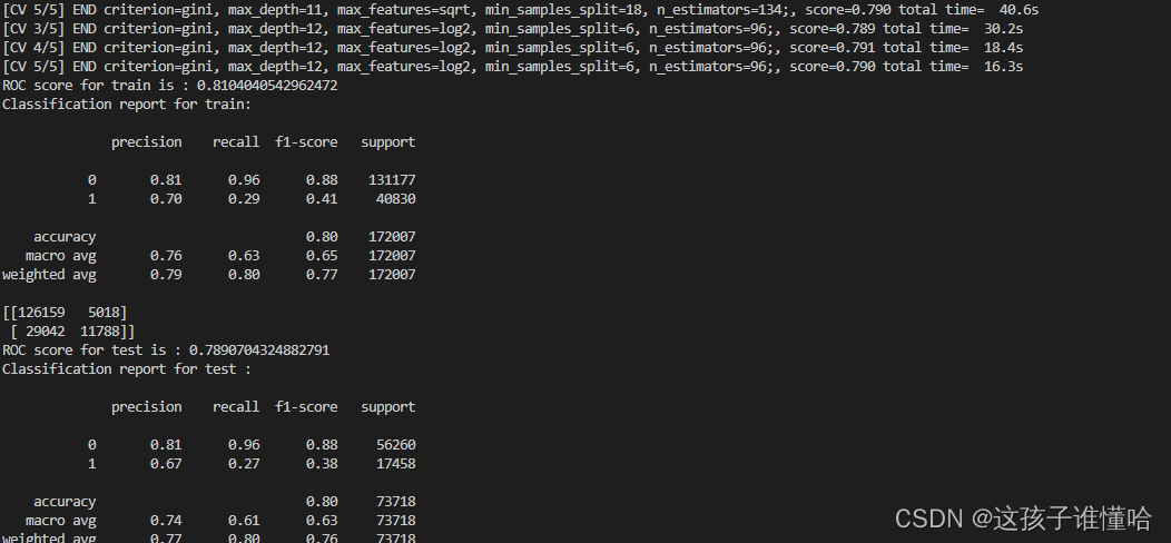
print(confusion_matrix(y_test, y_test_pred))# Tuning of lightgbm
lg = lgb.LGBMClassifier()
params = {'boosting_type':['gdbt', 'dart', 'rf'], 'max_depth':sp_randint(-1, 20), 'learning_rate':[0.1, 0.2,0.3,0.4,0.5], 'n_estimators':sp_randint(50, 400)}rscv = RandomizedSearchCV(lg, param_distributions=params, cv=5, scoring='roc_auc', n_iter=10, n_jobs=-1)
rscv.fit(x, y)
rscv.best_params_lg = lgb.LGBMClassifier(**rscv.best_params_)
lg.fit(x_train, y_train)y_train_pred = lg.predict(x_train)
y_train_prob = lg.predict_proba(x_train)[:, 1]print('ROC score for train is :', roc_auc_score(y_train, y_train_prob))
print('Classification report for train:\n')
print(classification_report(y_train, y_train_pred))
print(confusion_matrix(y_train, y_train_pred))y_test_pred = lg.predict(x_test)
y_test_prob = lg.predict_proba(x_test)[:, 1]print('ROC score for test is :', roc_auc_score(y_test, y_test_prob))
print('Classification report for test :\n')
print(classification_report(y_test, y_test_pred))
print(confusion_matrix(y_test, y_test_pred))sample_submission = df.iloc[:, [0]]
sample_submission['Is_Lead'] = lg.predict(df_test)
sample_submission.to_csv(r"C:\Users\Administrator\Desktop\DATA\Credit-Card-Lead-Prediction-main\sample_submission.csv")

简单的结果：