程序示例–局部加权线性回归
现在,我们在回归中又添加了 JLwr() 方法用于计算预测代价,以及 lwr() 方法用于完成局部加权线性回归:
# coding: utf-8
# linear_regression/regression.py# ...def JLwr(theta, X, y, x, c):"""局部加权线性回归的代价函数计算式Args:theta: 相关系数矩阵X: 样本集矩阵y: 标签集矩阵x: 待预测输入c: tauReturns:预测代价"""m,n = X.shapesummerize = 0for i in range(m):diff = (X[i]-x)*(X[i]-x).Tw = np.exp(-diff/(2*c*c))predictDiff = np.power(y[i] - X[i]*theta,2)summerize = summerize + w*predictDiffreturn summerize@exeTime
def lwr(rate, maxLoop, epsilon, X, y, x, c=1):"""局部加权线性回归Args:rate: 学习率maxLoop: 最大迭代次数epsilon: 预测精度X: 输入样本y: 标签向量x: 待预测向量c: tau"""m,n = X.shape# 初始化thetatheta = np.zeros((n,1))count = 0converged = Falseerror = float('inf')errors = []thetas = {}for j in range(n):thetas[j] = [theta[j,0]]# 执行批量梯度下降while count<=maxLoop:if(converged):breakcount = count + 1for j in range(n):deriv = (y-X*theta).T*X[:, j]/mtheta[j,0] = theta[j,0]+rate*derivthetas[j].append(theta[j,0])error = JLwr(theta, X, y, x, c)errors.append(error[0,0])# 如果已经收敛if(error < epsilon):converged = Truereturn theta,errors,thetas# ...
测试
# coding: utf-8
# linear_regression/test_lwr.py
import regression
import matplotlib.pyplot as plt
import matplotlib.ticker as mtick
import numpy as npif __name__ == "__main__":srcX, y = regression.loadDataSet('data/lwr.txt');m,n = srcX.shapesrcX = np.concatenate((srcX[:, 0], np.power(srcX[:, 0],2)), axis=1)# 特征缩放X = regression.standardize(srcX.copy())X = np.concatenate((np.ones((m,1)), X), axis=1)rate = 0.1maxLoop = 1000epsilon = 0.01predicateX = regression.standardize(np.matrix([[8, 64]]))predicateX = np.concatenate((np.ones((1,1)), predicateX), axis=1)result, t = regression.lwr(rate, maxLoop, epsilon, X, y, predicateX, 1)theta, errors, thetas = resultresult2, t = regression.lwr(rate, maxLoop, epsilon, X, y, predicateX, 0.1)theta2, errors2, thetas2 = result2# 打印特征点fittingFig = plt.figure()title = 'polynomial with bgd: rate=%.2f, maxLoop=%d, epsilon=%.3f'%(rate,maxLoop,epsilon)ax = fittingFig.add_subplot(111, title=title)trainingSet = ax.scatter(srcX[:, 0].flatten().A[0], y[:,0].flatten().A[0])print thetaprint theta2# 打印拟合曲线xx = np.linspace(1, 7, 50)xx2 = np.power(xx,2)yHat1 = []yHat2 = []for i in range(50):normalizedSize = (xx[i]-xx.mean())/xx.std(0)normalizedSize2 = (xx2[i]-xx2.mean())/xx2.std(0)x = np.matrix([[1,normalizedSize, normalizedSize2]])yHat1.append(regression.h(theta, x.T))yHat2.append(regression.h(theta2, x.T))fittingLine1, = ax.plot(xx, yHat1, color='g')fittingLine2, = ax.plot(xx, yHat2, color='r')ax.set_xlabel('temperature')ax.set_ylabel('yield')plt.legend([trainingSet, fittingLine1, fittingLine2], ['Training Set', r'LWR with $\tau$=1', r'LWR with $\tau$=0.1'])plt.show()# 打印误差曲线errorsFig = plt.figure()ax = errorsFig.add_subplot(111)ax.yaxis.set_major_formatter(mtick.FormatStrFormatter('%.2e'))ax.plot(range(len(errors)), errors)ax.set_xlabel('Number of iterations')ax.set_ylabel('Cost J')plt.show()
在测试程序中,我们分别对 τ τ τ 取值 0.1 和 1 ,得到了不同的拟合曲线: