（左边是数据集中的真图，右边是生成器生成的假图）

---

---

0. 特别提示

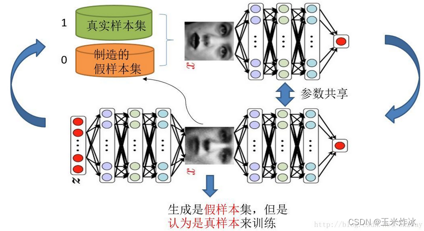
本文中的cgan是由dcgan简单修改和添加几行代码得到的（其实就是加上标签），以后都简称为cdcgan。建议你先掌握dcgan。

dcgan可以看我的这篇文章：【pytorch】基于mnist数据集的dcgan手写数字生成实现。

为什么不直接用cgan，而是在dcgan的基础上改？因为cgan训练的效果没有cdcgan好。这里给上github上znxlwm训练的对比图表。

mnist
对比项目	cgan	cdcgan
训练过程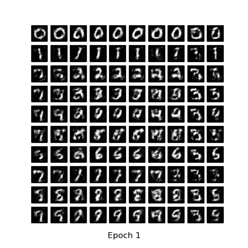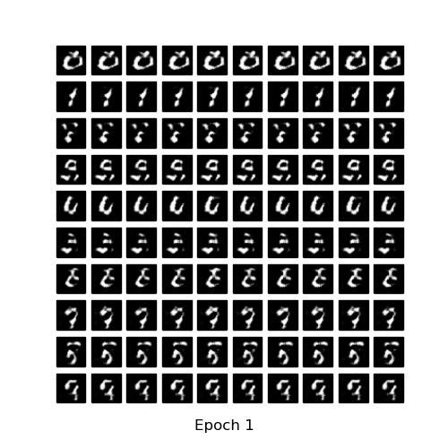
最终结果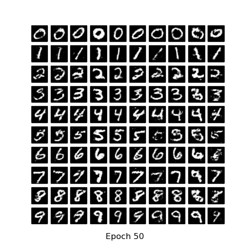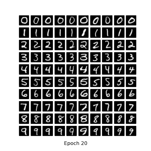
消耗时长	平均：9.13s/epoch；总长: 937.06s	平均：47.16s/epoch；总长: 1024.26s

1. 学习目标

本教程教你如何使用cdcgan（cgan+dcgan=cdcgan）训练mnist数据集，生成输出可控的手写数字。

2. 环境配置

2.1. Python

请参考官网安装。

2.2. Pytorch

请参考官网安装。

2.3. Jupyter notebook

pip install jupyter

2.4. Matplotlib

pip install matplotlib

3. 具体实现

3.1. 导入模块

import time
import torch
import torch.nn as nn
from torch.utils.data import DataLoader
from torchvision import utils, datasets, transforms
import matplotlib.pyplot as plt
import matplotlib.animation as animation
from IPython.display import HTML

3.2. 设置随机种子

设置随机种子，以便复现实验结果。

torch.manual_seed(0)

3.3. 超参数配置

• dataroot：存放数据集文件夹所在的路径
• workers ：数据加载器加载数据的线程数
• batch_size：训练的批次大小。
• image_size：训练图像的维度。默认是32x32。如果需要其它尺寸，必须更改$D$和$G$的结构，点击这里查看详情
• nc：输入图像的通道数。对于彩色图像是3
• num_classes：训练图像的类数。对于mnist数据集是10
• nz：潜在空间的长度
• ngf：与通过生成器进行的特征映射的深度有关
• ndf：设置通过鉴别器传播的特征映射的深度
• num_epochs：训练的总轮数。训练的轮数越多，可能会导致更好的结果，但也会花费更长的时间
• lr：学习率。DCGAN论文中用的是0.0002
• beta1：Adam优化器的参数beta1。论文中，值为0.5
• ngpus：可用的GPU数量。如果为0，代码将在CPU模式下运行；如果大于0，它将在该数量的GPU下运行

# Root directory for dataset
dataroot = "data/mnist"# Number of workers for dataloader
workers = 10# Batch size during training
batch_size = 100# Spatial size of training images. All images will be resized to this size using a transformer.
image_size = 32# Number of channels in the training images. For color images this is 3
nc = 1# Number of classes in the training images. For mnist dataset this is 10
num_classes = 10# Size of z latent vector (i.e. size of generator input)
nz = 100# Size of feature maps in generator
ngf = 64# Size of feature maps in discriminator
ndf = 64# Number of training epochs
num_epochs = 10# Learning rate for optimizers
lr = 0.0002# Beta1 hyperparam for Adam optimizers
beta1 = 0.5# Number of GPUs available. Use 0 for CPU mode.
ngpu = 1

3.4. 数据集

使用mnist数据集，其中训练集6万张，测试集1万张，我们这里不是分类任务，而是使用gan的生成任务，所以就不分训练和测试了，全部7万图像都可以利用。

train_data = datasets.MNIST(root=dataroot,train=True,transform=transforms.Compose([transforms.Resize(image_size),transforms.ToTensor(),transforms.Normalize((0.5,), (0.5,))]),download=True
)
test_data = datasets.MNIST(root=dataroot,train=False,transform=transforms.Compose([transforms.Resize(image_size),transforms.ToTensor(),transforms.Normalize((0.5,), (0.5,))])
)
dataset = train_data+test_data
print(f'Total Size of Dataset: {len(dataset)}')

输出：

Total Size of Dataset: 70000

注意：
这里作transforms.Normalize()标准化时必须使用(0.5,), (0.5,)而不是(0.1307,), (0.3081,)，否则会导致训练崩溃，生成器的loss不降反升。原因推测：生成器的最后一层加了tanh()激活函数会将数据归一化到[-1, 1]，也就是说“假图”的数据范围是[-1, 1]，那么真图也就是数据集的图片也应该归一化到此范围。我们知道transforms.ToTensor()操作将真图归一化到[0, 1]，如果再进行标准化，均值和标准差都取0.5，那么也就将真图的数据范围归一化到[-1, 1]了，和“假图”的数据范围一致。
$$\frac{min-mean}{std}=\frac{0-0.5}{0.5}=-1$$
$$\frac{max-mean}{std}=\frac{1-0.5}{0.5}=1$$

3.5. 数据加载器

num_workers设置为逻辑cpu个数即可，linux系统中查看逻辑cpu个数的命令：cat /proc/cpuinfo| grep "processor"| wc -l

dataloader = DataLoader(dataset=dataset,batch_size=batch_size,shuffle=True,num_workers=workers
)

3.6. 选择训练设备

检测cuda是否可用，可用就用cuda加速，否则使用cpu训练。

device = torch.device('cuda:0' if (torch.cuda.is_available() and ngpu > 0) else 'cpu')

3.7. 训练数据可视化

看看数据集中的训练数据长啥样。

imgs = {}
for x, y in dataset:if y not in imgs:imgs[y] = []elif len(imgs[y])!=10:imgs[y].append(x)elif sum(len(imgs[key]) for key in imgs)==100:breakelse:continueimgs = sorted(imgs.items(), key=lambda x:x[0])
imgs = [torch.stack(item[1], dim=0) for item in imgs]
imgs = torch.cat(imgs, dim=0)plt.figure(figsize=(10,10))
plt.title("Training Images")
plt.axis('off')
imgs = utils.make_grid(imgs, nrow=10)
plt.imshow(imgs.permute(1, 2, 0)*0.5+0.5)

3.8. 权重初始化

在dcgan论文中，作者指出所有模型权重应当从均值为0，标准差为0.02的正态分布中随机初始化。

def weights_init(m):classname = m.__class__.__name__if classname.find('Conv') != -1:nn.init.normal_(m.weight.data, 0.0, 0.02)elif classname.find('BatchNorm') != -1:nn.init.normal_(m.weight.data, 1.0, 0.02)nn.init.constant_(m.bias.data, 0)

3.9. 生成器

3.9.1. 生成器的结构

3.9.2. 构建生成器类

class Generator(nn.Module):def __init__(self, ngpu):super(Generator, self).__init__()self.ngpu = ngpuself.image = nn.Sequential(# state size. (nz) x 1 x 1nn.ConvTranspose2d(nz, ngf * 4, 4, 1, 0, bias=False),nn.BatchNorm2d(ngf * 4),nn.ReLU(True)# state size. (ngf*4) x 4 x 4)self.label = nn.Sequential(# state size. (num_classes) x 1 x 1nn.ConvTranspose2d(num_classes, ngf * 4, 4, 1, 0, bias=False),nn.BatchNorm2d(ngf * 4),nn.ReLU(True)# state size. (ngf*4) x 4 x 4)self.main = nn.Sequential(# state size. (ngf*8) x 4 x 4nn.ConvTranspose2d(ngf * 8, ngf * 4, 4, 2, 1, bias=False),nn.BatchNorm2d(ngf * 4),nn.ReLU(True),# state size. (ngf*4) x 8 x 8nn.ConvTranspose2d(ngf * 4, ngf * 2, 4, 2, 1, bias=False),nn.BatchNorm2d(ngf * 2),nn.ReLU(True),# state size. (ngf*2) x 16 x 16nn.ConvTranspose2d(ngf*2, nc, 4, 2, 1, bias=False),nn.Tanh()# state size. (nc) x 32 x 32)def forward(self, image, label):image = self.image(image)label = self.label(label)incat = torch.cat((image, label), dim=1)return self.main(incat)

3.9.3. 生成器实例化

# Create the generator
netG = Generator(ngpu).to(device)# Handle multi-gpu if desired
if device.type == 'cuda' and ngpu > 1:netG = nn.DataParallel(netG, list(range(ngpu)))# Apply the weights_init function to randomly initialize all weights to mean=0, stdev=0.2.
netG.apply(weights_init)

3.10. 判别器

3.10.1. 判别器的结构

3.10.2. 构建判别器类

class Discriminator(nn.Module):def __init__(self, ngpu):super(Discriminator, self).__init__()self.ngpu = ngpuself.image = nn.Sequential(# input is (nc) x 32 x 32nn.Conv2d(nc, ndf, 4, 2, 1, bias=False),nn.LeakyReLU(0.2, inplace=True)# state size. (ndf) x 16 x 16)self.label = nn.Sequential(# input is (num_classes) x 32 x 32nn.Conv2d(num_classes, ndf, 4, 2, 1, bias=False),nn.LeakyReLU(0.2, inplace=True)# state size. (ndf) x 16 x 16)self.main = nn.Sequential(# state size. (ndf*2) x 16 x 16nn.Conv2d(ndf * 2, ndf * 4, 4, 2, 1, bias=False),nn.BatchNorm2d(ndf * 4),nn.LeakyReLU(0.2, inplace=True),# state size. (ndf*4) x 8 x 8nn.Conv2d(ndf * 4, ndf * 8, 4, 2, 1, bias=False),nn.BatchNorm2d(ndf * 8),nn.LeakyReLU(0.2, inplace=True),# state size. (ndf*8) x 4 x 4nn.Conv2d(ndf * 8, 1, 4, 1, 0, bias=False),# state size. (1) x 1 x 1nn.Sigmoid())def forward(self, image, label):image = self.image(image)label = self.label(label)incat = torch.cat((image, label), dim=1)return self.main(incat)

3.10.3. 判别器实例化

# Create the Discriminator
netD = Discriminator(ngpu).to(device)# Handle multi-gpu if desired
if device.type == 'cuda' and ngpu > 1:netD = nn.DataParallel(netD, list(range(ngpu)))# Apply the weights_init function to randomly initialize all weights to mean=0, stdev=0.2.
netD.apply(weights_init)

3.11. 优化器和损失函数

# Initialize BCELoss function
criterion = nn.BCELoss()# Establish convention for real and fake labels during training
real_label_num = 1.
fake_label_num = 0.# Setup Adam optimizers for both G and D
optimizerD = torch.optim.Adam(netD.parameters(), lr=lr, betas=(beta1, 0.999))
optimizerG = torch.optim.Adam(netG.parameters(), lr=lr, betas=(beta1, 0.999))# Label one-hot for G
label_1hots = torch.zeros(10,10)
for i in range(10):label_1hots[i,i] = 1
label_1hots = label_1hots.view(10,10,1,1).to(device)# Label one-hot for D
label_fills = torch.zeros(10, 10, image_size, image_size)
ones = torch.ones(image_size, image_size)
for i in range(10):label_fills[i][i] = ones
label_fills = label_fills.to(device)# Create batch of latent vectors and laebls that we will use to visualize the progression of the generator
fixed_noise = torch.randn(100, nz, 1, 1).to(device)
fixed_label = label_1hots[torch.arange(10).repeat(10).sort().values]

3.12. 开始训练

# Lists to keep track of progress
img_list = []
G_losses = []
D_losses = []
D_x_list = []
D_z_list = []
loss_tep = 10print("Starting Training Loop...")
# For each epoch
for epoch in range(num_epochs):beg_time = time.time()# For each batch in the dataloaderfor i, data in enumerate(dataloader):############################# (1) Update D network: maximize log(D(x)) + log(1 - D(G(z)))############################# Train with all-real batchnetD.zero_grad()# Format batchreal_image = data[0].to(device)b_size = real_image.size(0)real_label = torch.full((b_size,), real_label_num).to(device)fake_label = torch.full((b_size,), fake_label_num).to(device)G_label = label_1hots[data[1]]D_label = label_fills[data[1]]# Forward pass real batch through Doutput = netD(real_image, D_label).view(-1)# Calculate loss on all-real batcherrD_real = criterion(output, real_label)# Calculate gradients for D in backward passerrD_real.backward()D_x = output.mean().item()## Train with all-fake batch# Generate batch of latent vectorsnoise = torch.randn(b_size, nz, 1, 1).to(device)# Generate fake image batch with Gfake = netG(noise, G_label)# Classify all fake batch with Doutput = netD(fake.detach(), D_label).view(-1)# Calculate D's loss on the all-fake batcherrD_fake = criterion(output, fake_label)# Calculate the gradients for this batcherrD_fake.backward()D_G_z1 = output.mean().item()# Add the gradients from the all-real and all-fake batcheserrD = errD_real + errD_fake# Update DoptimizerD.step()############################# (2) Update G network: maximize log(D(G(z)))###########################netG.zero_grad()# Since we just updated D, perform another forward pass of all-fake batch through Doutput = netD(fake, D_label).view(-1)# Calculate G's loss based on this outputerrG = criterion(output, real_label)# Calculate gradients for GerrG.backward()D_G_z2 = output.mean().item()# Update GoptimizerG.step()# Output training statsend_time = time.time()run_time = round(end_time-beg_time)print(f'Epoch: [{epoch+1:0>{len(str(num_epochs))}}/{num_epochs}]',f'Step: [{i+1:0>{len(str(len(dataloader)))}}/{len(dataloader)}]',f'Loss-D: {errD.item():.4f}',f'Loss-G: {errG.item():.4f}',f'D(x): {D_x:.4f}',f'D(G(z)): [{D_G_z1:.4f}/{D_G_z2:.4f}]',f'Time: {run_time}s',end='\r')# Save Losses for plotting laterG_losses.append(errG.item())D_losses.append(errD.item())# Save D(X) and D(G(z)) for plotting laterD_x_list.append(D_x)D_z_list.append(D_G_z2)# Save the Best Modelif errG < loss_tep:torch.save(netG.state_dict(), 'model.pt')loss_tep = errG# Check how the generator is doing by saving G's output on fixed_noise and fixed_labelwith torch.no_grad():fake = netG(fixed_noise, fixed_label).detach().cpu()img_list.append(utils.make_grid(fake, nrow=10))# Next lineprint()

输出：

Starting Training Loop...
Epoch: [01/10] Step: [700/700] Loss-D: 0.7205 Loss-G: 1.8315 D(x): 0.7095 D(G(z)): [0.2365/0.2161] Time: 115s
Epoch: [02/10] Step: [700/700] Loss-D: 1.3231 Loss-G: 2.0508 D(x): 0.7644 D(G(z)): [0.5831/0.1654] Time: 116s
Epoch: [03/10] Step: [700/700] Loss-D: 1.5194 Loss-G: 2.6285 D(x): 0.8626 D(G(z)): [0.6982/0.0936] Time: 110s
Epoch: [04/10] Step: [700/700] Loss-D: 0.8259 Loss-G: 1.4162 D(x): 0.6474 D(G(z)): [0.2771/0.2739] Time: 111s
Epoch: [05/10] Step: [700/700] Loss-D: 0.4708 Loss-G: 2.3000 D(x): 0.8081 D(G(z)): [0.1971/0.1272] Time: 111s
Epoch: [06/10] Step: [700/700] Loss-D: 0.3941 Loss-G: 3.5506 D(x): 0.9606 D(G(z)): [0.2575/0.0391] Time: 118s
Epoch: [07/10] Step: [700/700] Loss-D: 0.1330 Loss-G: 3.4693 D(x): 0.9434 D(G(z)): [0.0690/0.0441] Time: 113s
Epoch: [08/10] Step: [700/700] Loss-D: 0.0821 Loss-G: 4.5200 D(x): 0.9502 D(G(z)): [0.0279/0.0196] Time: 112s
Epoch: [09/10] Step: [700/700] Loss-D: 0.1145 Loss-G: 2.5075 D(x): 0.9040 D(G(z)): [0.0084/0.1038] Time: 111s
Epoch: [10/10] Step: [700/700] Loss-D: 0.3325 Loss-G: 2.9338 D(x): 0.8902 D(G(z)): [0.1730/0.0727] Time: 111s

3.13. 训练过程中的损失变化

plt.figure(figsize=(20, 10))
plt.title("Generator and Discriminator Loss During Training")
plt.plot(G_losses[::100], label="G")
plt.plot(D_losses[::100], label="D")
plt.xlabel("iterations")
plt.ylabel("Loss")
plt.axhline(y=0, label="0", c='g') # 渐近线（目标线）
plt.legend()

3.14. 训练过程中的D(x)和D(G(z))变化

plt.figure(figsize=(20, 10))
plt.title("D(x) and D(G(z)) During Training")
plt.plot(D_x_list[::100], label="D(x)")
plt.plot(D_z_list[::100], label="D(G(z))")
plt.xlabel("iterations")
plt.ylabel("Probability")
plt.axhline(y=0.5, label="0.5", c='g') # 渐近线（目标线）
plt.legend()

3.15. 可视化G的训练过程

fig = plt.figure(figsize=(10, 10))
plt.axis("off")
ims = [[plt.imshow(item.permute(1, 2, 0), animated=True)] for item in img_list]
ani = animation.ArtistAnimation(fig, ims, interval=1000, repeat_delay=1000, blit=True)
HTML(ani.to_jshtml())

4. 真图 vs 假图

# Size of the Figure
plt.figure(figsize=(20,10))# Plot the real images
plt.subplot(1,2,1)
plt.axis('off')
plt.title("Real Images")
imgs = utils.make_grid(imgs, nrow=10)
plt.imshow(imgs.permute(1, 2, 0)*0.5+0.5)# Load the Best Generative Model
netG = Generator(0)
netG.load_state_dict(torch.load('model.pt', map_location=torch.device('cpu')))
netG.eval()# Generate the Fake Images
with torch.no_grad():fake = netG(fixed_noise.cpu(), fixed_label.cpu())# Plot the fake images
plt.subplot(1,2,2)
plt.axis("off")
plt.title("Fake Images")
fake = utils.make_grid(fake, nrow=10)
plt.imshow(fake.permute(1, 2, 0)*0.5+0.5)# Save the comparation result
plt.savefig('comparation.jpg', bbox_inches='tight')

（左边是数据集中的真图，右边是生成器生成的假图）

5. 温馨提示

本教程使用的是1张GTX 1080 Ti的显卡，训练一个epoch大概113s左右。虽然实验室有8张卡，但没必要都用，亲测多卡训练速度反而更慢，当然我这里说的是数据并行DataParallel。分布式distributed训练的话应该会快很多，但对于初学者来说不太建议使用，因为配置很麻烦。如果你想使用分布式训练（ddp），那么建议你将此代码改为pytorch-lightning，因为它很好的支持ddp。

6. 完整代码

https://github.com/XavierJiezou/pytorch-cdcgan-mnist

7. 原始论文

Conditional Generative Adversarial Nets: https://arxiv.org/pdf/1411.1784.pdf

8. 引用参考

https://github.com/znxlwm/pytorch-MNIST-CelebA-cGAN-cDCGAN

9. 拓展阅读

本文中的神经网络结构图应该是用draw.io画的，下方是我用draw.io模仿的一部分：