首先,我们需要了解什么是“kNN”
kNN英文全称k Nearest Neighbor,即k近邻算法。
- 用途:分类问题
- kNN的工作原理:事先有一个有标签的样本数据集,然后输入没有标签的新数据后,将新数据的每个特征和样本集里的数据对应特征进行比较,最后算法提取样本集中特征最相似(最近邻)数据的分类标签。一般而言,只取k个最相似数据中出现次数最多的分类作为新数据的分类。
- 优点:精度高、对异常值不敏感、无数据输入假定。
- 缺点:计算复杂度高、空间复杂度高。
- 适用的数据范围:数值型和标称型。
一通文字理解下来后,下面给一个小例子
首先需要了解欧氏距离,很简单,就是平面上的两点之间的距离。
例:点A(x1, y1)与点B(x2, y2)之间的距离为
样本数据集
| 样本编号 | X | Y | label |
| 1 | 1.0 | 1.1 | A |
| 2 | 1.0 | 1.0 | A |
| 3 | 0 | 0 | B |
| 4 | 0 | 0.1 | B |

测试数据
| 编号 | X | Y | label |
| 1 | 0.1 | 0.1 | 待分类 |
从直观层面上就可以看出测试数据距离B类比较近,通过欧氏距离计算也是如此。下面给出kNN算法以及上面小例子的代码。
import numpy as np
import operator
import matplotlib.pyplot as pltdef kNN(inX, dataSet, labels, k):'''kNN算法:param inX: 需要分类的数据:param dataSet: 样本数据集:param labels: 样本数据的标签:param k: 需要取出的前k个:return: 最有可能的分类'''# 获取样本数据的个数dataSetSize = dataSet.shape[0]# np.tile函数将待分类的数据inX“广播”成和样本数据dataSet一样的形状# 获取待分类数据inX与样本数据集中的每个数据之间的差diffMat = np.tile(inX, (dataSetSize,1)) - dataSet# 平方sqDiffMat = diffMat**2# 按行累加sqDistances = sqDiffMat.sum(axis=1)# 开方,得出距离(欧氏距离)distances = sqDistances**0.5# 从小到大排序,得到的是数据的indexsortedDistIndicies = distances.argsort()classCount={}# 取出前k个距离最小的for i in range(k):voteIlabel = labels[sortedDistIndicies[i]]# 累计距离出现的次数,并做成字典classCount[voteIlabel] = classCount.get(voteIlabel,0) + 1# 将字典按值的大小排序,大的在前sortedClassCount = sorted(classCount.items(), key=operator.itemgetter(1), reverse=True)# 返回最有可能的预测值return sortedClassCount[0][0]def createDataSet():group = np.array([[1.0,1.1],[1.0,1.0],[0,0],[0,0.1]])labels = ['A','A','B','B']return group, labelsif __name__ == '__main__':group, labels = createDataSet()predict = kNN([0.1,0.1], group, labels, 3)print(predict) # 预测结果为B
接下来上实例,使用kNN算法改进约会网站的配对效果
数据集介绍:
总共10000条,包含三个特征(每年获得的飞行常客里程数,玩视频游戏所耗时间百分比,每周消费的冰淇淋公升数),而标签类型为(1代表“不喜欢的人”,2代表“魅力一般的人”,3代表“极具魅力的人”)
部分数据展示如下:(需要下载数据集的见文末)
40920	8.326976	0.953952	3
14488	7.153469	1.673904	2
26052	1.441871	0.805124	1
75136	13.147394	0.428964	1
样本数据集展示:

下面先给出作图代码,其他可以自主更换坐标轴以更好的分类:
def show():n = 1000 # number of points to createxcord1 = [];ycord1 = []xcord2 = [];ycord2 = []xcord3 = [];ycord3 = []markers = []colors = []fw = open('datingTestSet2.txt', 'w')for i in range(n):[r0, r1] = np.random.standard_normal(2)myClass = np.random.uniform(0, 1)if (myClass <= 0.16):fFlyer = np.random.uniform(22000, 60000)tats = 3 + 1.6 * r1markers.append(20)colors.append(2.1)classLabel = 1 # 'didntLike'xcord1.append(fFlyer);ycord1.append(tats)elif ((myClass > 0.16) and (myClass <= 0.33)):fFlyer = 6000 * r0 + 70000tats = 10 + 3 * r1 + 2 * r0markers.append(20)colors.append(1.1)classLabel = 1 # 'didntLike'if (tats < 0): tats = 0if (fFlyer < 0): fFlyer = 0xcord1.append(fFlyer);ycord1.append(tats)elif ((myClass > 0.33) and (myClass <= 0.66)):fFlyer = 5000 * r0 + 10000tats = 3 + 2.8 * r1markers.append(30)colors.append(1.1)classLabel = 2 # 'smallDoses'if (tats < 0): tats = 0if (fFlyer < 0): fFlyer = 0xcord2.append(fFlyer);ycord2.append(tats)else:fFlyer = 10000 * r0 + 35000tats = 10 + 2.0 * r1markers.append(50)colors.append(0.1)classLabel = 3 # 'largeDoses'if (tats < 0): tats = 0if (fFlyer < 0): fFlyer = 0xcord3.append(fFlyer);ycord3.append(tats)fw.close()fig = plt.figure()ax = fig.add_subplot(111)# ax.scatter(xcord,ycord, c=colors, s=markers)type1 = ax.scatter(xcord1, ycord1, s=20, c='red')type2 = ax.scatter(xcord2, ycord2, s=30, c='green')type3 = ax.scatter(xcord3, ycord3, s=50, c='blue')plt.rcParams['font.sans-serif'] = ['SimHei'] # 用来正常显示中文标签ax.legend([type1, type2, type3], ["不喜欢", "魅力一般", "极具魅力"], loc=2)ax.axis([-5000, 100000, -2, 25])plt.xlabel('每年获取的飞行常客里程数')plt.ylabel('玩游戏所耗时间百分比')plt.show()图像展示如下:

下面给出实例测试代码:
# 使用kNN算法改进约会网站的配对效果
import numpy as np
import pandas as pd
import operator
import matplotlib.pyplot as pltdef file_Matrix(filename):'''将源数据规整为所需要的数据形状:param filename: 源数据:return: returnMat:规整好的数据;classLabelVector:数据类标签'''data = pd.read_csv(filename, sep='\t').as_matrix()returnMat = data[:,0:3]classLabelVector = data[:,-1]return returnMat, classLabelVectordef autoNorm(dataSet):'''数据归一化:param dataSet::return:'''# 每列的最小值minVals = dataSet.min(0)# 每列的最大值maxVals = dataSet.max(0)ranges = maxVals - minVals# normDataSet = np.zeros(np.shape(dataSet))m = dataSet.shape[0]# np.tile(minVals,(m,1))的意思是将一行数据广播成m行normDataSet = (dataSet - np.tile(minVals, (m,1))) / np.tile(ranges, (m,1))# print(normDataSet)return normDataSet, ranges, minValsdef kNN(inX, dataSet, labels, k):'''kNN算法:param inX: 需要分类的数据:param dataSet: 样本数据集:param labels: 样本数据的标签:param k: 需要取出的前k个:return: 最有可能的分类'''# 获取样本数据的个数dataSetSize = dataSet.shape[0]# np.tile函数将待分类的数据inX“广播”成和样本数据dataSet一样的形状# 获取待分类数据inX与样本数据集中的每个数据之间的差diffMat = np.tile(inX, (dataSetSize,1)) - dataSet# 平方sqDiffMat = diffMat**2# 按行累加sqDistances = sqDiffMat.sum(axis=1)# 开方,得出距离(欧氏距离)distances = sqDistances**0.5# 从小到大排序,得到的是数据的indexsortedDistIndicies = distances.argsort()classCount={}# 取出前k个距离最小的for i in range(k):voteIlabel = labels[sortedDistIndicies[i]]# 累计距离出现的次数,并做成字典classCount[voteIlabel] = classCount.get(voteIlabel,0) + 1# 将字典按值的大小排序,大的在前sortedClassCount = sorted(classCount.items(), key=operator.itemgetter(1), reverse=True)# 返回最有可能的预测值return sortedClassCount[0][0]def datingClassTest():hoRatio = 0.10      #hold out 10%datingDataMat,datingLabels = file_Matrix('datingTestSet2.txt')       #load data setfrom filenormMat, ranges, minVals = autoNorm(datingDataMat)# print(normMat)m = normMat.shape[0]numTestVecs = int(m * hoRatio)errorCount = 0.0for i in range(numTestVecs):classifierResult = kNN(normMat[i,:],normMat[numTestVecs:m,:],datingLabels[numTestVecs:m],4)print("the classifier came back with: %d, the real answer is: %d" % (classifierResult, datingLabels[i]))if (classifierResult != datingLabels[i]): errorCount += 1.0print("测试集个数为%d ,分类错误的个数为%d"%(numTestVecs, errorCount))print("the total error rate is: %f" % (errorCount/float(numTestVecs)))print("accuracy: %f" % ((1-errorCount/float(numTestVecs))*100))if __name__ == '__main__':datingClassTest()
测试结果如下:
the classifier came back with: 2, the real answer is: 2
the classifier came back with: 1, the real answer is: 1
... ...
the classifier came back with: 1, the real answer is: 1
the classifier came back with: 2, the real answer is: 2
测试集个数为99 ,分类错误的个数为4
the total error rate is: 0.040404
accuracy: 95.959596测试的结果是错误率为4.04%,可以接受。不过还可以自主调节hoRatio和变量k的值,以便让错误率降低。
数据集下载:(百度网盘)
链接:https://pan.baidu.com/s/1UErV8D4Hrw557tjj9fyjlQ
提取码:o80d
参考文献:《Machine Learning in Action》