SIFT特征点提取算法

1、算法简介

尺度不变特征转换即SIFT (Scale-invariant feature transform)是一种计算机视觉的算法。它用来侦测与描述影像中的局部性特征，它在空间尺度中寻找极值点，并提取出其位置、尺度、旋转不变量，此算法由 David Lowe在1999年所发表，2004年完善总结。

其应用范围包含物体辨识、机器人地图感知与导航、影像缝合、3D模型建立、手势辨识、影像追踪和动作比对。

局部影像特征的描述与侦测可以帮助辨识物体，SIFT特征是基于物体上的一些局部外观的兴趣点而与影像的大小和旋转无关。对于光线、噪声、细微视角改变的容忍度也相当高。基于这些特性，它们是高度显著而且相对容易撷取，在母数庞大的特征数据库中，很容易辨识物体而且鲜有误认。使用 SIFT特征描述对于部分物体遮蔽的侦测率也相当高，甚至只需要3个以上的SIFT物体特征就足以计算出位置与方位。在现今的电脑硬件速度下和小型的特征数据库条件下，辨识速度可接近即时运算。SIFT特征的信息量大，适合在海量数据库中快速准确匹配。

SIFT算法的实质是在不同的尺度空间上查找关键点(特征点)，并计算出关键点的方向。SIFT所查找到的关键点是一些十分突出，不会因光照，仿射变换和噪音等因素而变化的点，如角点、边缘点、暗区的亮点及亮区的暗点等。

2、算法实施

以下代码均来自rmislam复现的SIFT代码，github地址。rmislam将SIFT分为了以下数个步骤，封装在computeKeypointsAndDescriptors()函数中，每一步分别用代码进行实现，接下来会逐代码分析SIFT算法的原理。

def computeKeypointsAndDescriptors(image, sigma=1.6, num_intervals=3, assumed_blur=0.5, image_border_width=5):image = image.astype('float32')base_image = generateBaseImage(image, sigma, assumed_blur)num_octaves = computeNumberOfOctaves(base_image.shape)gaussian_kernels = generateGaussianKernels(sigma, num_intervals)gaussian_images = generateGaussianImages(base_image, num_octaves, gaussian_kernels)dog_images = generateDoGImages(gaussian_images)keypoints = findScaleSpaceExtrema(gaussian_images, dog_images, num_intervals, sigma, image_border_width)keypoints = removeDuplicateKeypoints(keypoints)keypoints = convertKeypointsToInputImageSize(keypoints)descriptors = generateDescriptors(keypoints, gaussian_images)return keypoints, descriptors

generateBaseImage() 适当地模糊和加倍输入图像以生成图像金字塔的基础图像
computeNumberOfOctaves() 来计算图像金字塔中的层数octaves
generateGaussianKernels() 开始创建一个尺度列表（高斯核大小）
该列表传递给 generateGaussianImages()，它反复模糊和下采样基础图像。
减去相邻的高斯图像对以形成高斯差分DoG图像的金字塔
findScaleSpaceExtrema() 识别关键点
通过删除重复项并将它们转换为输入图像大小来清理这些关键点。
通过 generateDescriptors() 为每个关键点生成描述符。

2.1 generateBaseImage()

SIFT算法中定义图像自身和尺度空间分别为 $I (x, y)$ 和 $L(x,y,\sigma)$ ，则尺度空间计算公式如下：
$L(x,y,\sigma)=I(x,y)*G(x,y,\sigma)$

$G(x,y,\sigma)=\frac{1}{2\pi\sigma^2}e^{-(x^2+y^2)/2\sigma^2}$

其中*指的是在 $x$ 和 $y$ 方向进行卷积操作， $\sigma$ 表示尺度空间坐标。

def generateBaseImage(image, sigma, assumed_blur):"""Generate base image from input image by upsampling by 2 in both directions and blurring"""image = resize(image, (0, 0), fx=2, fy=2, interpolation=INTER_LINEAR)sigma_diff = sqrt(max((sigma ** 2) - ((2 * assumed_blur) ** 2), 0.01))return GaussianBlur(image, (0, 0), sigmaX=sigma_diff, sigmaY=sigma_diff)  # the image blur is now sigma instead of assumed_blur

generateBaseImage()的作用是对输入图像进行升采样并应用高斯模糊。在高斯模糊阶段，假设输入图像的模糊度为assistant_blur = 0.5（这里设置assistant_blur 为0.5是因为相机已对图像进行 $\sigma=0.5$ 的模糊），如果我们希望得到的基础图像的模糊度为sigma，需要通过sigma_diff 对输入图像进行模糊处理。通过内核大小 $\sigma_1$ 模糊输入图像，然后通过 $\sigma_2$ 模糊，结果图像相当于仅通过 $\sigma$ 模糊输入图像一次，其中 $\sigma^2=\sigma_1^2+\sigma_2^2$ ，证明过程见这里。

GaussianBlur(src,ksize,sigmaX,dst= None,sigmaY= None,borderType= None)，其中各参数解释如下:

src:输入图像
ksize:(核的宽度,核的高度)，输入高斯核的尺寸，核的宽高都必须是正奇数。否则，将会从参数sigma中计算得到。
dst:输出图像，尺寸与输入图像一致。
sigmaX:高斯核在X方向上的标准差。sigmaY:高斯核在Y方向上的标准差。默认为None，如果sigmaY=0，则它将被设置为与sigmaX相等的值。如果这两者都为0,则它们的值会从ksize中计算得到。

2.2 computeNumberOfOctaves()

def computeNumberOfOctaves(image_shape):"""Compute number of octaves in image pyramid as function of base image shape (OpenCV default)"""return int(round(log(min(image_shape)) / log(2) - 1))

computeNumberOfOctaves()函数用来计算图像金字塔的层数，计算公式为 $O=[log_2min(M,N)]-t,t\in[0,log_2\{\min(M,N)\}]$

2.3 generateGaussianKernels()

每一个Octave有6个Intvrval尺寸相同但模糊系数 $\sigma$ 不同的采用图像组成，其变化公式为：
$\sigma(o,r)=\sigma_02^{o+\frac{r}{s}}\qquad o\in [0,\dots,O-1],r\in[0,\dots,s+2]$
其中 $o$ 为组索引序号， $r$ 为层索引序号， $s$ 为高斯差分金字塔每组层数， $s = 3$ ， $O$ 为金字塔组数， $\sigma_0$ 为高斯模糊初始值，取 $k$ 为总层数的倒数，即 $k=2^{\frac{1}{S}}$ ，在构建高斯金字塔时，层内每组的尺度坐标按如下公式计算：
$\sigma(s)=\sqrt{(k^s\sigma_0)^2-(k^{s-1}\sigma_0)^2}$
在计算组内某一层图像的尺度时，直接使用如下公式进行计算：
$\sigma(r)=\sigma_02^{\frac{r}{s}}\qquad r\in[0,\dots,s+2]$

def generateGaussianKernels(sigma, num_intervals):"""Generate list of gaussian kernels at which to blur the input image. Default values of sigma, intervals, and octaves follow section 3 of Lowe's paper."""num_images_per_octave = num_intervals + 3k = 2 ** (1. / num_intervals)gaussian_kernels = zeros(num_images_per_octave)  # scale of gaussian blur necessary to go from one blur scale to the next within an octavegaussian_kernels[0] = sigmafor image_index in range(1, num_images_per_octave):sigma_previous = (k ** (image_index - 1)) * sigmasigma_total = k * sigma_previousgaussian_kernels[image_index] = sqrt(sigma_total ** 2 - sigma_previous ** 2)return gaussian_kernels

GaussianKernels()函数为特定层中的每个图像创建一个模糊量 $\sigma$ 的列表。图像金字塔有 numOctaves 层，但每个层本身都有 numIntervals + 3 个图像。同一层中的所有图像具有相同的宽度和高度，但模糊量依次增加。

用从一倍到两倍blur value的numIntervals生成其中numIntervals + 1个图像。
剩下2个图像分别是在第一步模糊的第一张图像和这层中模糊后的最后一张图像。

在这里插入图片描述

需要这两张图像的原因是因为需要减去相邻的高斯图像来创建一个 DoG 图像金字塔。

2.4 generateGaussianImages()

为保证高斯差分金字塔的尺度空间（高斯模糊系数）的连续性，下一个Octave(i+1)的第一层由上一个Octave(i)的倒数第三层直接降采样不需要模糊产生。

def generateGaussianImages(image, num_octaves, gaussian_kernels):"""Generate scale-space pyramid of Gaussian images"""gaussian_images = []for octave_index in range(num_octaves):gaussian_images_in_octave = []gaussian_images_in_octave.append(image)  # first image in octave already has the correct blurfor gaussian_kernel in gaussian_kernels[1:]:image = GaussianBlur(image, (0, 0), sigmaX=gaussian_kernel, sigmaY=gaussian_kernel)gaussian_images_in_octave.append(image)gaussian_images.append(gaussian_images_in_octave)octave_base = gaussian_images_in_octave[-3]image = resize(octave_base, (int(octave_base.shape[1] / 2), int(octave_base.shape[0] / 2)), interpolation=INTER_NEAREST)return array(gaussian_images)

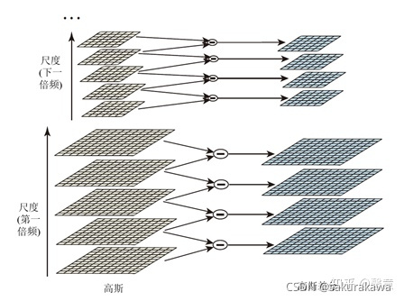
2.5 generateDoGImages()

2002年Mikolajczyk在详细的实验比较中发现尺度归一化的高斯拉普拉斯函数 $\sigma^2\bigtriangledown^2G$ 的极大值和极小值同其它的特征提取函数，而Lindeberg早在1994年就发现高斯差分函数（DOG算子）与尺度归一化的高斯拉普拉斯函数 $\sigma^2\bigtriangledown^2G$ 非常近似， $G(x,y,k\sigma)-G(x,y,\sigma)\approx(k-1)\sigma^2\bigtriangledown^2G$ 。

在这里插入图片描述

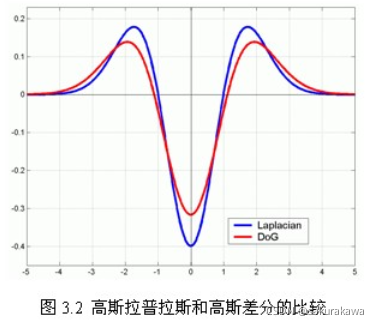
红色曲线表示的是高斯差分算子，而蓝色曲线表示的是高斯拉普拉斯算子。Lowe使用更高效的高斯差分算子代替拉普拉斯算子进行极值检测，如下：
$D(x,y,\sigma)=(G(x,y,k\sigma)-G(x,y,\sigma))*I(x,y)\\ =L(x,y,k\sigma)-L(x,y,\sigma)$
在实际计算时，使用高斯金字塔每组中相邻上下两层图像相减，得到高斯差分图像，进行极值检测。

def generateDoGImages(gaussian_images):"""Generate Difference-of-Gaussians image pyramid"""dog_images = []for gaussian_images_in_octave in gaussian_images:dog_images_in_octave = []for first_image, second_image in zip(gaussian_images_in_octave, gaussian_images_in_octave[1:]):dog_images_in_octave.append(subtract(second_image, first_image))  # ordinary subtraction will not work because the images are unsigned integersdog_images.append(dog_images_in_octave)return array(dog_images)

在这里插入图片描述

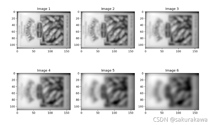
高斯金字塔第三层的图像

在这里插入图片描述

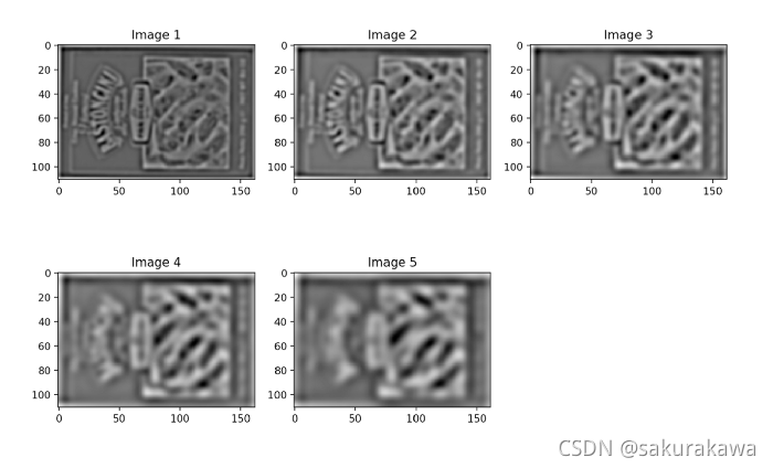
差分高斯金字塔第三层的图像

2.6 findScaleSpaceExtrema()

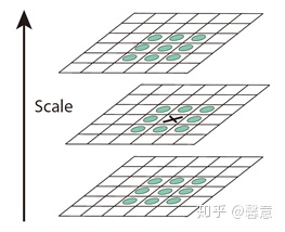
在函数findScaleSpaceExtrema()中，对每一层进行遍历，一次遍历一层中三个连续的图像。函数 isPixelAnExtremum()寻找大于或小于所有 26 个相邻像素的像素：中间图像中有 8 个相邻像素，下邻图中有 9 个相邻像素，上邻图中有 9 个相邻像素。

在这里插入图片描述

当找到一个极值时，使用 localizeExtremumViaQuadraticFit() 沿所有三个维度（宽度、高度和比例）在子像素级别定位它的位置。

def findScaleSpaceExtrema(gaussian_images, dog_images, num_intervals, sigma, image_border_width, contrast_threshold=0.04):"""Find pixel positions of all scale-space extrema in the image pyramid"""threshold = floor(0.5 * contrast_threshold / num_intervals * 255)  # from OpenCV implementationkeypoints = []for octave_index, dog_images_in_octave in enumerate(dog_images):for image_index, (first_image, second_image, third_image) in enumerate(zip(dog_images_in_octave, dog_images_in_octave[1:], dog_images_in_octave[2:])):# (i, j) is the center of the 3x3 arrayfor i in range(image_border_width, first_image.shape[0] - image_border_width):for j in range(image_border_width, first_image.shape[1] - image_border_width):if isPixelAnExtremum(first_image[i-1:i+2, j-1:j+2], second_image[i-1:i+2, j-1:j+2], third_image[i-1:i+2, j-1:j+2], threshold):localization_result = localizeExtremumViaQuadraticFit(i, j, image_index + 1, octave_index, num_intervals, dog_images_in_octave, sigma, contrast_threshold, image_border_width)if localization_result is not None:keypoint, localized_image_index = localization_resultkeypoints_with_orientations = computeKeypointsWithOrientations(keypoint, octave_index, gaussian_images[octave_index][localized_image_index])for keypoint_with_orientation in keypoints_with_orientations:keypoints.append(keypoint_with_orientation)return keypoints

2.6.1 localizeExtremumViaQuadraticFit()

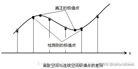
以上方法检测到的极值点是离散空间的极值点，以下通过拟合三维二次函数来精确确定关键点的位置和尺度，同时去除低对比度的关键点和不稳定的边缘响应点(因为DoG算子会产生较强的边缘响应)，以增强匹配稳定性、提高抗噪声能力。离散空间的极值点并不是真正的极值点，下图显示了二维函数离散空间得到的极值点与连续空间极值点的差别。利用已知的离散空间点插值得到的连续空间极值点的方法叫做子像素插值。

在这里插入图片描述

为了提高关键点的稳定性，需要对尺度空间DoG函数进行曲线插值。利用DoG函数在尺度空间的Taylor展开式(插值函数)，任意一极值点在 $X_0=(x_0,y_0,\sigma_0)$ 处舍掉二阶以后的项的结果为：
$f\left(\left[\begin{matrix}x\\y\\\sigma\end{matrix}\right]\right)\approx f\left(\left[\begin{matrix}x_0\\y_0\\\sigma_0\end{matrix}\right]\right)+\left[\frac{\partial f}{\partial x} \ \frac{\partial f}{\partial x} \ \frac{\partial f}{\partial x}\right]\left(\left[\begin{matrix}x\\y\\\sigma\end{matrix}\right]-\left[\begin{matrix}x_0\\y_0\\\sigma_0\end{matrix}\right]\right)+\\ \frac{1}{2}([\begin{matrix}x& y& \sigma\end{matrix}]-[\begin{matrix}x_0& y_0& \sigma_0\end{matrix}])\left[\begin{matrix}\frac{\partial ^2f}{\partial x\partial x}& \frac{\partial ^2f}{\partial x\partial y}& \frac{\partial ^2f}{\partial x\partial \sigma} \\ \frac{\partial ^2f}{\partial x\partial y}& \frac{\partial ^2f}{\partial y\partial y}& \frac{\partial ^2f}{\partial y\partial \sigma}\\ \frac{\partial ^2f}{\partial x\partial \sigma}& \frac{\partial ^2f}{\partial y\partial \sigma}& \frac{\partial ^2f}{\partial \sigma \partial \sigma}\end{matrix}\right]\left(\left[\begin{matrix}x\\y\\\sigma\end{matrix}\right]-\left[\begin{matrix}x_0\\y_0\\\sigma_0\end{matrix}\right]\right)$
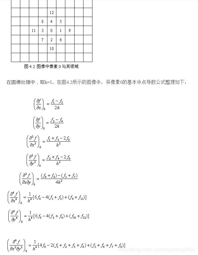
其中 $f$ 的一阶偏导数，二阶偏导数，以及二阶混合偏导数由下面几个公式 $（ h = 1 ）$ 得
$\frac{\partial f}{\partial x}=\frac{f(i,j+1)-f(i,j-1)}{2h},\ \frac{\partial f}{\partial y}=\frac{f(i+1,j)-f(i-1,j)}{2h}\\ \frac{\partial ^2 f}{\partial x^2}=\frac{f(i,j+1)-f(i,j-1)-2f(i,j)}{h^2},\ \frac{\partial ^2 f}{\partial y^2}=\frac{f(i+1,j)-f(i-1,j)-2f(i,j)}{h^2}\\ \frac{\partial ^2 f}{\partial x\partial y}=\frac{f(i-1,j-1)+f(i+1,j+1)-f(i-1,j+1)-f(i+1,j-1)}{4h^2}$
上述算式的矩阵表示如下：
$D(X)=D+\frac{\partial D^T}{\partial X}X+\frac{1}{2}X^T\frac{\partial ^2 D}{\partial X^2}X$
其中，X求导并让方程等于零，可以得到极值点的偏移量为：
$\hat{X}=-\frac{\partial ^2 D^{-1}}{\partial X^2}\frac{\partial D}{\partial X}$
对应极值点，方程的值为：
$D(\hat{X})=D+\frac{1}{2}\frac{\partial D^T}{\partial X}\hat{X}$
其中, $\hat{X}$ 代表相对插值中心的偏移量，当它在任一维度上的偏移量大于0.5时，意味着插值中心已经偏移到它的邻近点上，所以必须改变当前关键点的位置。同时在新的位置上反复插值直到收敛；也有可能超出所设定的迭代次数或者超出图像边界的范围，此时这样的点应该删除，在Lowe中进行了5次迭代。另外，过小的点易受噪声的干扰而变得不稳定，所以将小于某个经验值(Lowe论文中使用0.03，rmislam实现时使用0.04/S)的极值点删除。同时，在此过程中获取特征点的精确位置(原位置加上拟合的偏移量)以及尺度 $\sigma$ 。

def localizeExtremumViaQuadraticFit(i, j, image_index, octave_index, num_intervals, dog_images_in_octave, sigma, contrast_threshold, image_border_width, eigenvalue_ratio=10, num_attempts_until_convergence=5):"""Iteratively refine pixel positions of scale-space extrema via quadratic fit around each extremum's neighbors"""logger.debug('Localizing scale-space extrema...')extremum_is_outside_image = Falseimage_shape = dog_images_in_octave[0].shapefor attempt_index in range(num_attempts_until_convergence):# need to convert from uint8 to float32 to compute derivatives and need to rescale pixel values to [0, 1] to apply Lowe's thresholdsfirst_image, second_image, third_image = dog_images_in_octave[image_index-1:image_index+2]pixel_cube = stack([first_image[i-1:i+2, j-1:j+2],second_image[i-1:i+2, j-1:j+2],third_image[i-1:i+2, j-1:j+2]]).astype('float32') / 255.gradient = computeGradientAtCenterPixel(pixel_cube)hessian = computeHessianAtCenterPixel(pixel_cube)extremum_update = -lstsq(hessian, gradient, rcond=None)[0]if abs(extremum_update[0]) < 0.5 and abs(extremum_update[1]) < 0.5 and abs(extremum_update[2]) < 0.5:breakj += int(round(extremum_update[0]))i += int(round(extremum_update[1]))image_index += int(round(extremum_update[2]))# make sure the new pixel_cube will lie entirely within the imageif i < image_border_width or i >= image_shape[0] - image_border_width or j < image_border_width or j >= image_shape[1] - image_border_width or image_index < 1 or image_index > num_intervals:extremum_is_outside_image = Truebreakif extremum_is_outside_image:logger.debug('Updated extremum moved outside of image before reaching convergence. Skipping...')return Noneif attempt_index >= num_attempts_until_convergence - 1:logger.debug('Exceeded maximum number of attempts without reaching convergence for this extremum. Skipping...')return NonefunctionValueAtUpdatedExtremum = pixel_cube[1, 1, 1] + 0.5 * dot(gradient, extremum_update)if abs(functionValueAtUpdatedExtremum) * num_intervals >= contrast_threshold:xy_hessian = hessian[:2, :2]xy_hessian_trace = trace(xy_hessian)xy_hessian_det = det(xy_hessian)if xy_hessian_det > 0 and eigenvalue_ratio * (xy_hessian_trace ** 2) < ((eigenvalue_ratio + 1) ** 2) * xy_hessian_det:# Contrast check passed -- construct and return OpenCV KeyPoint objectkeypoint = KeyPoint()keypoint.pt = ((j + extremum_update[0]) * (2 ** octave_index), (i + extremum_update[1]) * (2 ** octave_index))keypoint.octave = octave_index + image_index * (2 ** 8) + int(round((extremum_update[2] + 0.5) * 255)) * (2 ** 16)keypoint.size = sigma * (2 ** ((image_index + extremum_update[2]) / float32(num_intervals))) * (2 ** (octave_index + 1))  # octave_index + 1 because the input image was doubledkeypoint.response = abs(functionValueAtUpdatedExtremum)return keypoint, image_indexreturn None

一个定义不好的高斯差分算子的极值在横跨边缘的地方有较大的主曲率，而在垂直边缘的方向有较小的主曲率。DOG算子会产生较强的边缘响应，需要剔除不稳定的边缘响应点。获取特征点处的Hessian矩阵，主曲率通过一个2x2的Hessian矩阵H求出（D的主曲率和H的特征值成正比）：
$H=\left[\begin{matrix}D_{xx}& D_{xy} \\ D_{xy}&D_{yy}\end{matrix}\right]$
假设H的特征值为 $\alpha$ 和 $\beta$ （ $\alpha$ ， $\beta$ （代表x和y方向的梯度）且 $\alpha>\beta$ 。令 $\alpha=r\beta$ 则有：
$Tr(H)=D_{xx}+D_{yy}=\alpha+\beta \ , Det(H)=D_{xx}D_{yy}-(D_{xy})^2=\alpha\beta$
其中 $T r (H)$ 求取H的对角元素和； $D e t (H)$ 为求H的行列式值，则
$\frac{Tr(H)^2}{Det(H)}=\frac{(\alpha+\beta)^2}{\alpha\beta}=\frac{(r\beta+\beta)^2}{r\beta^2}=\frac{(r+1)^2}{r}$
则公式 $\frac{(r+1)^2}{r}$ 的值在两个特征值相等时最小，随着的增大而增大。值越大，说明两个特征值的比值越大，即在某一个方向的梯度值越大，而在另一个方向的梯度值越小，而边缘恰恰就是这种情况。所以为了剔除边缘响应点，需要让该比值小于一定的阈值，因此，为了检测主曲率是否在某域值 $r$ 下，只需检测:
$\frac{Tr(H)^2}{Det(H)}<\frac{(r+1)^2}{r}$
论文建议 $r = 10$ ，OpenCv也采用 $r = 10$ ，rmislam在复现时也采用 $r = 10$ 。

2.6.2 computeKeypointsWithOrientations()

为了使描述符具有旋转不变性，需要利用图像的局部特征为给每一个关键点分配一个基准方向。使用图像梯度的方法求取局部结构的稳定方向。对于在 DOG 金字塔中检测出的关键点点，采集其所在高斯金字塔图像3σ领域窗口内像素的梯度和方向分布特征。梯度的模值和方向如下：
$m(x,y)=\sqrt{(L(x+1,y)-L(x-1,y))^2+(L(x,y+1)-L(x,y-1))^2}\\ \theta(x,y)=tan^{-1}\frac{L(x,y+1)-L(x,y-1)}{L(x+1,y)-L(x-1,y)}$
其中，L为关键点所在的尺度空间值，按Lowe的建议，梯度的模值 $m (x, y)$ 按 $σ=1.5σ_{oct}$ 的高斯分布加成，按尺度采样的 $3 σ$ 原则，领域窗口半径为 $3*1.5σ_oct$ 。

def computeKeypointsWithOrientations(keypoint, octave_index, gaussian_image, radius_factor=3, num_bins=36, peak_ratio=0.8, scale_factor=1.5):"""Compute orientations for each keypoint"""logger.debug('Computing keypoint orientations...')keypoints_with_orientations = []image_shape = gaussian_image.shapescale = scale_factor * keypoint.size / float32(2 ** (octave_index + 1))  # compare with keypoint.size computation in localizeExtremumViaQuadraticFit()radius = int(round(radius_factor * scale))weight_factor = -0.5 / (scale ** 2)raw_histogram = zeros(num_bins)smooth_histogram = zeros(num_bins)for i in range(-radius, radius + 1):region_y = int(round(keypoint.pt[1] / float32(2 ** octave_index))) + iif region_y > 0 and region_y < image_shape[0] - 1:for j in range(-radius, radius + 1):region_x = int(round(keypoint.pt[0] / float32(2 ** octave_index))) + jif region_x > 0 and region_x < image_shape[1] - 1:dx = gaussian_image[region_y, region_x + 1] - gaussian_image[region_y, region_x - 1]dy = gaussian_image[region_y - 1, region_x] - gaussian_image[region_y + 1, region_x]gradient_magnitude = sqrt(dx * dx + dy * dy)gradient_orientation = rad2deg(arctan2(dy, dx))weight = exp(weight_factor * (i ** 2 + j ** 2))  # constant in front of exponential can be dropped because we will find peaks laterhistogram_index = int(round(gradient_orientation * num_bins / 360.))raw_histogram[histogram_index % num_bins] += weight * gradient_magnitudefor n in range(num_bins):smooth_histogram[n] = (6 * raw_histogram[n] + 4 * (raw_histogram[n - 1] + raw_histogram[(n + 1) % num_bins]) + raw_histogram[n - 2] + raw_histogram[(n + 2) % num_bins]) / 16.orientation_max = max(smooth_histogram)orientation_peaks = where(logical_and(smooth_histogram > roll(smooth_histogram, 1), smooth_histogram > roll(smooth_histogram, -1)))[0]for peak_index in orientation_peaks:peak_value = smooth_histogram[peak_index]if peak_value >= peak_ratio * orientation_max:# Quadratic peak interpolation# The interpolation update is given by equation (6.30) in https://ccrma.stanford.edu/~jos/sasp/Quadratic_Interpolation_Spectral_Peaks.htmlleft_value = smooth_histogram[(peak_index - 1) % num_bins]right_value = smooth_histogram[(peak_index + 1) % num_bins]interpolated_peak_index = (peak_index + 0.5 * (left_value - right_value) / (left_value - 2 * peak_value + right_value)) % num_binsorientation = 360. - interpolated_peak_index * 360. / num_binsif abs(orientation - 360.) < float_tolerance:orientation = 0new_keypoint = KeyPoint(*keypoint.pt, keypoint.size, orientation, keypoint.response, keypoint.octave)keypoints_with_orientations.append(new_keypoint)return keypoints_with_orientations

在完成关键点的梯度计算后，使用直方图统计领域内像素的梯度和方向。梯度直方图将0~360度的方向范围分为36个柱(bins)，其中每柱10度。在将梯度的模值累加到直方图时，注意需要乘以一个高斯权重，即 $m(x,y)=m(x,y)*G(x,y,1.5\sigma)$ ，这里 $x, y$ 为局部坐标。

为了防止某个梯度方向角度因受到噪声的干扰而突变，我们还需要对梯度方向直方图进行平滑处理。在这里使用了和OpenCV一样的平滑公式，Opencv 所使用的平滑公式为：
$H(i)=\frac{h(i-2)+h(i+2)}{16}+\frac{4\times (h(i-1)+h(i+1))}{16}+\frac{6\times h(i)}{16}$
其中 $i \in [0, 35]$ , $h$ 和 $H$ 分别表示平滑前和平滑后的直方图。由于角度是循环的，即 $0^0=360^0$ ，如果出现 $h (j)$ ， $j$ 超出了 $(0, \dots, 35)$ 的范围，那么可以通过圆周循环的方法找到它所对应的、在 $0^0=360^0$ 之间的值，如 $h (- 1) = h (35)$ 。

方向直方图的峰值则代表了该特征点处邻域梯度的方向，以直方图中最大值作为该关键点的主方向。为了增强匹配的鲁棒性，只保留峰值大于主方向峰值80％的方向作为该关键点的辅方向。因此，对于同一梯度值的多个峰值的关键点位置，在相同位置和尺度将会有多个关键点被创建但方向不同。仅有15％的关键点被赋予多个方向，但可以明显的提高关键点匹配的稳定性。实际编程实现中，就是把该关键点复制成多份关键点，并将方向值分别赋给这些复制后的关键点，并且，离散的梯度方向直方图要进行插值拟合处理，来求得更精确的方向角度值。

在进行差值拟合时，我们只在主方向以及负方向所在的柱子序号 $j$ 且满足 $KaTeX parse error: Undefined control sequence: \and at position 12: H(j)>H(j-1)\̲a̲n̲d̲ ̲H(j)>h(j+1)$ 的 $j-1,\ j \ ,j+1$ 柱子进行差值，三个点可以确定一条抛物线。假设我们在第 $i$ 个小柱子上找一个精确地方向，那么由上述分析知道，设差值抛物线方程为 $h(i)=at^2+bt+c$ ，其中 $a, b, c$ 为抛物线的系数， $t$ 为自变量且 $t\in[-1,1]$ ，此抛物线求导并令其等于0，即 $h (t)^{'} = 0$ 得 $t_{max}=-\frac{b}{2a}$ 。将三个插值点带入方程可得：
$\left\{ \begin{array}{lr} h(-1)=a-b+c \\ h(0)=c \\ h(1)=a+b+c \end{array} \right. \Rightarrow \left\{ \begin{array}{lr} a=\frac{h(1)+h(-1)}{2}-h(0) \\ b=\frac{h(1)-h(-1)}{2} \\ c=h(0) \end{array} \right.$
由上式知：
$t_{max}=-\frac{b}{2a}=\frac{h(-1)-h(1)}{2[h(-1)+h(1)-2h(0)]}\\ i'=i+\frac{h(i-1)-h(i+1)}{2[h(i-1)+h(i+1)-2h(i)]}$
其中， $t_{max}$ 为局部坐标系中的取值， $i^{'}$ 为柱子在直方图中的索引号。

2.7 generateDescriptors()

通过以上步骤，对于每一个关键点，拥有三个信息：位置(pt)、尺度(size)以及方向(orientation)。接下来就是为每个关键点建立一个描述符，使其不随各种变化而改变，比如光照变化、视角变化等等。并且描述符应该有较高的独特性，以便于提高特征点正确匹配的概率。

将关键点附近的区域划分为 $d * d$ (Lowe建议 $d = 4$ )个子区域，每个子区域作为一个种子点，每个种子点有8个方向。考虑到实际计算时，需要采用三线性插值，所需图像窗口边长为 $3\times 3\times σ_{oct}(d+1)$ 。在考虑到旋转因素(方便下一步将坐标轴旋转到关键点的方向)，实际计算所需的图像区域半径为：
$radius=\frac{3\sigma_{oct}\times \sqrt{2}\times (d+1)}{2}$
计算结果四舍五入取整。之后将坐标轴旋转为关键点的方向，以确保旋转不变性。旋转后邻域内采样点的新坐标为：
$\left(\begin{matrix} x' \\ y'\end{matrix} \right)= \left(\begin{matrix} cos\theta & -sin\theta\\sin\theta & cos\theta\end{matrix} \right)\quad (x,y\in[-radius,radius])$
之后将邻域内的采样点分配到对应的子区域内，将子区域内的梯度值分配到8个方向上，计算其权值。

旋转后的采样点坐标在半径为radius的圆内被分配到 $d\times d$ 的子区域，计算影响子区域的采样点的梯度和方向，分配到8个方向上。

旋转后的采样点 $(x^{'}, y^{'})$ 落在子区域的下标为：
$\left(\begin{matrix} x'' \\ y''\end{matrix} \right)= \frac{1}{3\sigma_{oct}}\left(\begin{matrix} x' \\ y'\end{matrix} \right)+\frac{d}{2}$
Lowe建议子区域的像素的梯度大小按 $\sigma=0.5d$ 的高斯加权计算，即：
$w=m(a+x,b+y)*e^{-\frac{(x')^2+(y')^2}{2\times (0.5d)^2}}$
其中a，b为关键点在高斯金字塔图像中的位置坐标。实际计算r时，使用的区域为 $d + 1$ ，在实际计算时+0.5，保证四舍五入，加而不减保证参加统计的数据尽可能多，同时为了平衡，在计算 $(x^{''}, y^{''})$ 时-0.5。

def unpackOctave(keypoint):"""Compute octave, layer, and scale from a keypoint"""octave = keypoint.octave & 255layer = (keypoint.octave >> 8) & 255if octave >= 128:octave = octave | -128scale = 1 / float32(1 << octave) if octave >= 0 else float32(1 << -octave)return octave, layer, scaledef generateDescriptors(keypoints, gaussian_images, window_width=4, num_bins=8, scale_multiplier=3, descriptor_max_value=0.2):"""Generate descriptors for each keypoint"""logger.debug('Generating descriptors...')descriptors = []for keypoint in keypoints:octave, layer, scale = unpackOctave(keypoint)gaussian_image = gaussian_images[octave + 1, layer]num_rows, num_cols = gaussian_image.shapepoint = round(scale * array(keypoint.pt)).astype('int')bins_per_degree = num_bins / 360.angle = 360. - keypoint.anglecos_angle = cos(deg2rad(angle))sin_angle = sin(deg2rad(angle))weight_multiplier = -0.5 / ((0.5 * window_width) ** 2)row_bin_list = []col_bin_list = []magnitude_list = []orientation_bin_list = []histogram_tensor = zeros((window_width + 2, window_width + 2, num_bins))   # first two dimensions are increased by 2 to account for border effects# Descriptor window size (described by half_width) follows OpenCV conventionhist_width = scale_multiplier * 0.5 * scale * keypoint.sizehalf_width = int(round(hist_width * sqrt(2) * (window_width + 1) * 0.5))   # sqrt(2) corresponds to diagonal length of a pixelhalf_width = int(min(half_width, sqrt(num_rows ** 2 + num_cols ** 2)))     # ensure half_width lies within imagefor row in range(-half_width, half_width + 1):for col in range(-half_width, half_width + 1):row_rot = col * sin_angle + row * cos_anglecol_rot = col * cos_angle - row * sin_anglerow_bin = (row_rot / hist_width) + 0.5 * window_width - 0.5col_bin = (col_rot / hist_width) + 0.5 * window_width - 0.5if row_bin > -1 and row_bin < window_width and col_bin > -1 and col_bin < window_width:window_row = int(round(point[1] + row))window_col = int(round(point[0] + col))if window_row > 0 and window_row < num_rows - 1 and window_col > 0 and window_col < num_cols - 1:dx = gaussian_image[window_row, window_col + 1] - gaussian_image[window_row, window_col - 1]dy = gaussian_image[window_row - 1, window_col] - gaussian_image[window_row + 1, window_col]gradient_magnitude = sqrt(dx * dx + dy * dy)gradient_orientation = rad2deg(arctan2(dy, dx)) % 360weight = exp(weight_multiplier * ((row_rot / hist_width) ** 2 + (col_rot / hist_width) ** 2))row_bin_list.append(row_bin)col_bin_list.append(col_bin)magnitude_list.append(weight * gradient_magnitude)orientation_bin_list.append((gradient_orientation - angle) * bins_per_degree)for row_bin, col_bin, magnitude, orientation_bin in zip(row_bin_list, col_bin_list, magnitude_list, orientation_bin_list):# Smoothing via trilinear interpolation# Notations follows https://en.wikipedia.org/wiki/Trilinear_interpolation# Note that we are really doing the inverse of trilinear interpolation here (we take the center value of the cube and distribute it among its eight neighbors)row_bin_floor, col_bin_floor, orientation_bin_floor = floor([row_bin, col_bin, orientation_bin]).astype(int)row_fraction, col_fraction, orientation_fraction = row_bin - row_bin_floor, col_bin - col_bin_floor, orientation_bin - orientation_bin_floorif orientation_bin_floor < 0:orientation_bin_floor += num_binsif orientation_bin_floor >= num_bins:orientation_bin_floor -= num_binsc1 = magnitude * row_fractionc0 = magnitude * (1 - row_fraction)c11 = c1 * col_fractionc10 = c1 * (1 - col_fraction)c01 = c0 * col_fractionc00 = c0 * (1 - col_fraction)c111 = c11 * orientation_fractionc110 = c11 * (1 - orientation_fraction)c101 = c10 * orientation_fractionc100 = c10 * (1 - orientation_fraction)c011 = c01 * orientation_fractionc010 = c01 * (1 - orientation_fraction)c001 = c00 * orientation_fractionc000 = c00 * (1 - orientation_fraction)histogram_tensor[row_bin_floor + 1, col_bin_floor + 1, orientation_bin_floor] += c000histogram_tensor[row_bin_floor + 1, col_bin_floor + 1, (orientation_bin_floor + 1) % num_bins] += c001histogram_tensor[row_bin_floor + 1, col_bin_floor + 2, orientation_bin_floor] += c010histogram_tensor[row_bin_floor + 1, col_bin_floor + 2, (orientation_bin_floor + 1) % num_bins] += c011histogram_tensor[row_bin_floor + 2, col_bin_floor + 1, orientation_bin_floor] += c100histogram_tensor[row_bin_floor + 2, col_bin_floor + 1, (orientation_bin_floor + 1) % num_bins] += c101histogram_tensor[row_bin_floor + 2, col_bin_floor + 2, orientation_bin_floor] += c110histogram_tensor[row_bin_floor + 2, col_bin_floor + 2, (orientation_bin_floor + 1) % num_bins] += c111descriptor_vector = histogram_tensor[1:-1, 1:-1, :].flatten()  # Remove histogram borders# Threshold and normalize descriptor_vectorthreshold = norm(descriptor_vector) * descriptor_max_valuedescriptor_vector[descriptor_vector > threshold] = thresholddescriptor_vector /= max(norm(descriptor_vector), float_tolerance)# Multiply by 512, round, and saturate between 0 and 255 to convert from float32 to unsigned char (OpenCV convention)descriptor_vector = round(512 * descriptor_vector)descriptor_vector[descriptor_vector < 0] = 0descriptor_vector[descriptor_vector > 255] = 255descriptors.append(descriptor_vector)return array(descriptors, dtype='float32')

在这里插入图片描述

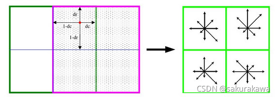
将所得采样点在子区域中的下标(图中蓝色窗口内红色点)线性插值，计算其对每个种子点的贡献。则最终累加在每个方向上的梯度大小为：
$weight=|grad(I_{\sigma}(x,y))|\times e^{-\frac{x_k^2+y_k^2}{2\sigma_w}} \times (1-d_r)\times (1-d_c) \times(1-d_o)$
其中， $x_k$ 为该点与关键点的列距离， $y_k$ 为该点与关键点的行距离， $\sigma_w$ 等于描述子窗口宽度 $\frac{3\sigma d}{2}$ 。

如上统计的 $4 * 4 * 8 = 128$ 个梯度信息即为该关键点的特征向量。特征向量形成后，为了去除光照变化的影响，需要对它们进行归一化处理，对于图像灰度值整体漂移，图像各点的梯度是邻域像素相减得到，所以也能去除。得到的描述子向量为 $H=(h_1,h_2,...,h_{128})$ ，归一化后的特征向量为 $L=(L_1,L_2,......,L_{128})$ ，则：
$L_j=\frac{h_j}{\sum\limits_{i=1}^{128}h_i},\quad j=1,2,3...$
描述子向量门限。非线性光照，相机饱和度变化对造成某些方向的梯度值过大，而对方向的影响微弱。因此设置门限值(向量归一化后，一般取0.2，代码中取0.2)截断较大的梯度值。然后，再进行一次归一化处理，提高特征的鉴别性。