Kernel Density (KD)

Feinman R., Curtin R. R., Shintre S. and Gardner A. B. Detecting Adversarial Samples from Artifacts. arXiv preprint arXiv:1703.00410, 2017.

原文代码

作者认为普通样本的特征和对抗样本的特征位于不同的流形中, 故可以通过密度估计的方法, 估计出普通样本的密度函数, 然后求得样本各自的置信度, 选择合适的阈值(通过ROC-AUC之类的), 便有了区分普通样本和对抗样本的方法.

假设
$$z=h(x)\in {\mathbb{R}}^d.$$
为将样本$x$提取为特征$z$

1. 选取合适的样本数目$x_1,\cdots ,x_N$;
2. 提取特征$z_1,\cdots ,z_N$;
3. 构建核密度估计函数:
   $$\begin{gathered} \hat{f}(x)=\frac{1}{N}\sum _{i=1}^N{k}_{\sigma }(z_i,h(x)), \\ {k}_{\sigma }(z,z^{\prime })=\frac{1}{(2\pi {)}^{\frac{d}{2}}{\sigma }^d}\exp (-\frac{\Vert z^{\prime }-z{\Vert }^2}{2{\sigma }^2}). \end{gathered}$$

选择合适的阈值$t$, 对于样本$x$, 判定其为对抗样本, 若$\hat{f}(x)<t$.

有些时候, 可以对每一类构建一个$\hat{f}(x)$, 但这个情况也就只能用在ROC-AUC了.

Local Intrinsic Dimensionality (LID)

LID

Gaussian Discriminant Analysis (GDA)

Lee K., Lee K., Lee H. and Shin J. A simple unified framework for detecting out-of-distribution samples and adversarial attacks. In Advances in Neural Information Processing Systems (NIPS), 2018.

原文代码

作者假设特征$z=h(x)$(所属类别为$c$)满足后验分布:
$$z|y=c\sim \mathcal{N}({\mu }_c,\Sigma ),$$
即
$$p(h(x)|y=c)=\mathcal{N}(h(x)|{\mu }_c,\Sigma ),$$
注意到对于不同的$c$, 协方差矩阵$\Sigma$是一致的(这个假设是为了便于直接用于分类, 但是与detection无关, 便不多赘述).

均值和协方差矩阵通过如下方式估计:
$${\hat{\mu }}_c=\frac{1}{N_c}\sum _{i:y_i=c}h(x_i),\hat{\Sigma }=\frac{1}{N}\sum _c\sum _{i:y_i=c}(h(x_i)-{\hat{\mu }}_c)(h(x_i)-{\hat{\mu }}_c{)}^T.$$

故可以用
$$\hat{f}(x):=\underset{c}{\max }\mathcal{N}(h(x)|{\hat{\mu }}_c,\hat{\Sigma }),$$
来区分$x$是否为abnormal的样本(对抗的或者偏离训练分布的样本).

在文中用的是log化(且去掉比例系数)的指标:
$$M(x)=\underset{c}{\max }-(h(x)-{\hat{\mu }}_c{)}^T\hat{\Sigma }(h(x)-{\hat{\mu }}_c).$$

改方法可以进一步拓展(实际上光用这个指标看实验结果似乎并不理想):

1. Input pre-processing:

对于输入的样本进行如下变换:
$$\hat{x}=x+ϵ\mathrm{s}\mathrm{i}\mathrm{g}\mathrm{n}({\nabla }_{x}M(x)).$$
有点像fgsm生成对抗样本, 但感觉这么做的原因是让$\hat{f}(x)$之间的区别大一点.

2. Feature ensemble:

即对不同层的特征$h_l(x)$都进行如上的操作, 然后得到${\hat{f}}_1,\cdots ,{\hat{f}}_L$, 并通过SVM来训练得到权重${\alpha }_l$, 最后的score为
$$\sum _l\alpha {\hat{f}}_l(x).$$

注: 文中实际为$M_l(x)$.

Gaussian Mixture Model (GMM)

Zheng Z. and Hong P. Robust detection of adversarial attacks by modeling the intrinsic properties of deep neural networks. In Advances in Neural Information Processing Systems (NIPS), 2018.

类似的, 对于特征$z=h(x)$, 假设其服从GMM:
$$p(h(x)|y=c;\theta )=\sum _{k=1}^K{w}_i\mathcal{N}(h(x)|{\mu }_{ck},{\Sigma }_{ck}),$$
并用EM算法来估计.

注: 对每一个类别都需要估计一个GMM模型.

于是
$${\hat{f}}_c(x)=p(h(x)|y=c;\theta ),$$
当其小于给定的threshold的时候, 便认为其不属于类别$c$.

问: 所以当所有的$c$都被拒绝的时候, 就可以认为是对抗样本了?

SelectiveNet

Geilman Y., El-Yaniv R. SelectiveNet: A deep neural network with an integrated reject option. In International Conference on Machine Learning (ICML), 2019.

原文代码

本文的模型解释起来有点复杂, 在一个普通的判别网络$f$的基础上:
$$(f,g)(x):=\{\begin{array}{ll}f(x)& \text{if }g(x)=1,\\ \text{don’t know}& \text{if }g(x)=0.\end{array}$$
其中$g$是一个用来选择是否判断的模块.
作者给出了两个指标:

Coverage:
$$\varphi (g):=E_P[g(x)],$$
以及
Selective Risk:
$$R(f,g):=\frac{E_P[\ell (f(x),y)g(x)]}{\varphi (g)}.$$
Coverage不能太低, 因为如果全部拒绝判断模型就没有意义了, 然后$R(f,g)$自然是越低越好, 但是注意到, 虽然一味拒绝回答能够使得分子接近0, 但是分母也会接近0, 所以需要一个平衡.
二者的经验估计如下:
$$\begin{gathered} \hat{r}(f,g|S_N):=\frac{\frac{1}{N}{\sum }_{i=1}^N\ell (f(x_i),y_i)g(x_i)}{\varphi (g|S_N)}, \\ \varphi (g|S_N):=\frac{1}{N}\sum _{i=1}^{N}g(x_i). \end{gathered}$$

注: 在实际使用中, $g$的取值往往在$[0,1]$间, 此时可以选取threshold t来选择是否判断.

作者设计了一个结构如下:

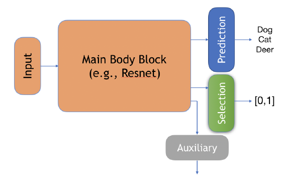
其中:
Prediction: $f$;
Selection: $g$;
Auxiliary: $h$, 作者说此为别的任务来帮助训练的.

最后的损失:
$$\begin{gathered} \mathcal{L}=\alpha {\mathcal{L}}_{(f,g)}+(1-\alpha ){\mathcal{L}}_h \\ {\mathcal{L}}_{(f,g)}={\hat{r}}_{\ell }(f,g|S_N)+\lambda \Psi (c-\hat{\varphi }(g|S_N)) \\ \Psi (a)=\max (0,a{)}^2 \\ {\mathcal{L}}_h=\hat{r}(h|S_N)=\frac{1}{N}\sum _{i=1}^N\ell (h(x_i),y_i). \end{gathered}$$

Combined Abstention Robustness Learning (CARL)

Laidlaw C., Feizi S. Playing it safe: adversarial robustness with an abstain option. arXiv preprint arXiv:1911.11253, 2019.

原文代码

假设$f$将样本$x$映射为 Y ⋃ { a } \mathcal{Y} \bigcup \{a\} Y⋃{a}, 其中$a$表示弃权(don’t know).

则我们可以定义:
R n a t ( f ) : = E ( x , y ) ∼ D 1 { f ( x ) ≠ y } R a d v ( f ) : = E ( x , y ) ∼ D max ⁡ x ~ ∈ B ϵ ( x ) 1 { f ( x ~ ≠ y and  f ( x ~ ) ≠ a } . \mathcal{R}_{nat} (f) := \mathbb{E}_{(x, y) \sim \mathcal{D}} \mathbf{1}\{f(x) \not = y\} \\ \mathcal{R}_{adv}(f) := \mathbb{E}_{(x, y) \sim \mathcal{D}} \max_{\tilde{x} \in \mathcal{B}_{\epsilon}(x)} \mathbf{1}\{f(\tilde{x} \not = y \text{ and } f(\tilde{x}) \not = a\}. Rnat​(f):=E(x,y)∼D​1{f(x)​=y}Radv​(f):=E(x,y)∼D​x~∈Bϵ​(x)max​1{f(x~​=y and f(x~)​=a}.

很自然的, 我们可以通过优化下列损失
$$\mathcal{R}(f)={\mathcal{R}}_{nat}(f)+c{\mathcal{R}}_{adv}(f),$$
来获得一个带有弃权功能的判别器. 并且通过权重$c$我们可以选择更好的natural精度或者更保守但更加安全的策略.

直接优化上面的损失是困难的, 故选择损失来替换. 作者采用普通的交叉熵损失来代替nat:
$${\mathcal{L}}_{nat}(f)={\mathbb{E}}_{(x,y)\sim \mathcal{D}}-\log p_y(x),$$
用下列之一替代adv:
L a d v ( f ) E ( x , y ) ∼ D max ⁡ x ~ ∈ B ϵ ( x ) ℓ ( f , x ~ , y ) , ℓ = { ℓ ( 1 ) , ℓ ( 2 ) } ℓ ( 1 ) = − log ⁡ ( p y ( x ~ ) + p a ( x ~ ) ) ℓ ( 2 ) = ( − log ⁡ ( p y ( x ~ ) ) ⋅ ( − log ⁡ p a ( x ~ ) ) \mathcal{L}_{adv}(f) \mathbb{E}_{(x, y) \sim \mathcal{D}} \max_{\tilde{x} \in \mathcal{B}_{\epsilon}(x)} \ell(f, \tilde{x}, y), \\ \ell = \{\ell^{(1)}, \ell^{(2)}\} \\ \ell^{(1)} = -\log (p_y (\tilde{x}) + p_a (\tilde{x})) \\ \ell^{(2)} = (-\log (p_y (\tilde{x})) \cdot (-\log p_a (\tilde{x})) \\ Ladv​(f)E(x,y)∼D​x~∈Bϵ​(x)max​ℓ(f,x~,y),ℓ={ℓ(1),ℓ(2)}ℓ(1)=−log(py​(x~)+pa​(x~))ℓ(2)=(−log(py​(x~))⋅(−logpa​(x~))

Adversarial Training with a Rejection Option

Kato M., Cui Z., Fukuhara Y. ATRO: Adversarial training with a rejection option. arXiv preprint arXiv:2010.12905, 2020.

凸relax.

Energy-based Out-of-distribution Detection

Liu W., Wang X., Owens J. D., Li Y. Energy-based out-of-distribution detection. In Advances in Neural Information Processing Systems (NIPS), 2020.

普通的softmax分类网络可以从energy-based model的角度考虑:
$$\begin{gathered} p(y|x)=\frac{e^{-E(x,y)/T}}{{\int }_{y^{\prime }}{e}^{-E(x,y^{\prime })/T}}, \\ E(x,y)=-f_y(x), \end{gathered}$$
Helmholtz free energy:
$$E(x;f):=-T\cdot \log {\int }_{y^{\prime }}{e}^{-E(x,y^{\prime })/T}=-T\cdot \log \sum _i^K{e}^{f_i(x)}/T.$$

实际上, 通过$E(x;f)$我们可以构建$x$的能量模型:
$$p(x)=\frac{e^{-E(x;f)/T}}{{\int }_x{e}^{-E(x;f)/T}},$$
故我们可以通过$p(x)$来判断一个样本是不是OOD的.

特别的, 由于对于所有的$x$
$$Z={\int }_x{e}^{-E(x;f)/T}$$
都是一致的, 所以我们只需要比较
$$e^{-E(x;f)/T}$$
的大小就可以了.

特别的, 作者指出为什么用$p(y|x)$来作为判断是否OOD的依据不合适:
$$\begin{array}{ll}\log {\max }_{y}p(y|x)& =\log {\max }_y\frac{e^{f_y(x)}}{{\sum }_i{e}^{f_i(x)}}\\ & =\log \frac{e^{f_{\max }(x)}}{{\sum }_i{e}^{f_i(x)}}\\ & =E(x;f(x)-f^{\max }(x))\\ & =E(x;f)+f^{max}(x)\\ & =-\log p(x)+f^{max}(x)-\log Z\\ & /\propto -\log p(x).\end{array}$$

WOW!

Confidence-Calibrated Adversarial Training: Generalizing to Unseen Attacks (CCAT)

Stutz D., Hein M. and Schiele B. Confidence-calibrated adversarial training: generalizing to unseen attacks. In International Conference on Machine Learning (ICML), 2020.

原文代码

假设$f(x)$为预测的概率向量, CCAT通过如下算法优化:

1. 输入: $(x_1,y_1),\cdots ,(x_B,y_B)$;
2. 将其中一半用于对抗训练, 一半用于普通训练:
   $$\min \sum _{b=1}^{B/2}\mathcal{L}(f({\tilde{x}}_b,{\tilde{y}}_b))+\sum _{b=B/2+1}^B\mathcal{L}(f(x_b),y_b).$$
3. 其中
   $$\begin{gathered} {\tilde{x}}_b=x_b+{\delta }_b, \\ {\tilde{y}}_b=\lambda ({\delta }_b)\text{ one\_hot}(y_b)+(1-\lambda ({\delta }_b))\frac{1}{K}, \\ {\delta }_b=\underset{{\delta }_{\infty }\le ϵ}{\mathrm{argmax}}\underset{k\ne y_b}{\max }{f}_k(x_b+\delta ), \\ \lambda ({\delta }_b):=(1-\min (1,\frac{\Vert {\delta }_b{\Vert }_{\infty }}{ϵ}){)}^{\rho }. \end{gathered}$$

$\tilde{y}$是真实标签和均匀分布的一个凸组合, 这个还是挺有道理的.

最后, 倘若如果
$$\underset{k}{\max }{f}_k(x),$$
即置信度比较小的话, 拒绝判断(这个可靠的原因是目标函数让对抗样本趋于均匀分布).