一、Meshgrid函数

import numpy as np
import matplotlib.pyplot as pltx = np.linspace(0, 1, 5)
y = np.linspace(0, 1, 3)
print("x = ", x)
print("-" * 50)
print("y = ", y)
print("-" * 100)X, Y = np.meshgrid(x, y)
print("\nX.shape = {0} \nX = \n{1}".format(X.shape, X))
print("-" * 50)
print("Y.shape = {0} \nY = \n{1}".format(Y.shape, Y))
print("-" * 100)

打印结果：

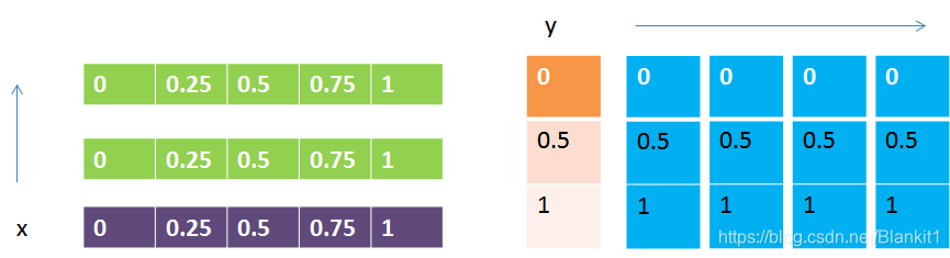
x =  [0.   0.25 0.5  0.75 1.  ]
--------------------------------------------------
y =  [0.  0.5 1. ]
----------------------------------------------------------------------------------------------------X.shape = (3, 5) 
X = 
[[0.   0.25 0.5  0.75 1.  ][0.   0.25 0.5  0.75 1.  ][0.   0.25 0.5  0.75 1.  ]]
--------------------------------------------------
Y.shape = (3, 5) 
Y = 
[[0.  0.  0.  0.  0. ][0.5 0.5 0.5 0.5 0.5][1.  1.  1.  1.  1. ]]
----------------------------------------------------------------------------------------------------Process finished with exit code 0

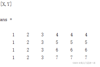
meshgrid函数的运行过程，可以通过下面的示意图来加深理解：

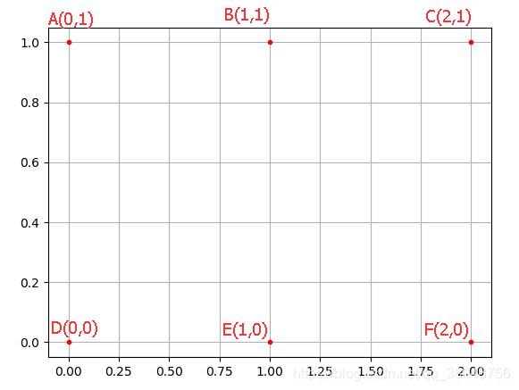
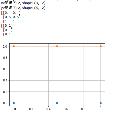
再者，也可以通过在matplotlib中进行可视化，来查看函数运行后得到的网格化数据的结果

import numpy as np
import matplotlib.pyplot as pltx = np.linspace(0, 1, 5)
y = np.linspace(0, 1, 3)
print("x = ", x)
print("-" * 50)
print("y = ", y)
print("-" * 100)X, Y = np.meshgrid(x, y)
print("\nX.shape = {0} \nX = \n{1}".format(X.shape, X))
print("-" * 50)
print("Y.shape = {0} \nY = \n{1}".format(Y.shape, Y))
print("-" * 100)plt.plot(X, Y, marker='.', color='blue', linestyle='none')
plt.show()

当然，我们也可以获得网格平面上坐标点的数据，如下：

import numpy as np
import matplotlib.pyplot as pltx = np.linspace(0, 1, 5)
y = np.linspace(0, 1, 3)
print("x = ", x)
print("-" * 50)
print("y = ", y)
print("-" * 100)X, Y = np.meshgrid(x, y)
print("\nX.shape = {0} \nX = \n{1}".format(X.shape, X))
print("-" * 50)
print("Y.shape = {0} \nY = \n{1}".format(Y.shape, Y))
print("-" * 100)z = [i for i in zip(X.flat, Y.flat)]
print("z = {0}".format(z))

打印结果：

x =  [0.   0.25 0.5  0.75 1.  ]
--------------------------------------------------
y =  [0.  0.5 1. ]
----------------------------------------------------------------------------------------------------X.shape = (3, 5) 
X = 
[[0.   0.25 0.5  0.75 1.  ][0.   0.25 0.5  0.75 1.  ][0.   0.25 0.5  0.75 1.  ]]
--------------------------------------------------
Y.shape = (3, 5) 
Y = 
[[0.  0.  0.  0.  0. ][0.5 0.5 0.5 0.5 0.5][1.  1.  1.  1.  1. ]]
----------------------------------------------------------------------------------------------------
z = [(0.0, 0.0), (0.25, 0.0), (0.5, 0.0), (0.75, 0.0), (1.0, 0.0), (0.0, 0.5), (0.25, 0.5), (0.5, 0.5), (0.75, 0.5), (1.0, 0.5), (0.0, 1.0), (0.25, 1.0), (0.5, 1.0), (0.75, 1.0), (1.0, 1.0)]Process finished with exit code 0

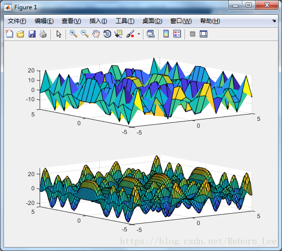
二、Meshgrid函数的一些应用场景

Meshgrid函数常用的场景有等高线绘制及机器学习中SVC超平面的绘制（二维场景下）。

1、等高线

import tensorflow as tfimport matplotlib.pyplot as pltdef func(x):""":param x: [b, 2]:return:"""z = tf.math.sin(x[..., 0]) + tf.math.sin(x[..., 1])return zx = tf.linspace(0., 2 * 3.14, 500)
y = tf.linspace(0., 2 * 3.14, 500)
# [50, 50]
point_x, point_y = tf.meshgrid(x, y)
# [50, 50, 2]
points = tf.stack([point_x, point_y], axis=2)
# points = tf.reshape(points, [-1, 2])
print('points:', points.shape)
z = func(points)
print('z:', z.shape)plt.figure('plot 2d func value')
plt.imshow(z, origin='lower', interpolation='none')
plt.colorbar()plt.figure('plot 2d func contour')
plt.contour(point_x, point_y, z)
plt.colorbar()
plt.show()

打印结果：

points: (500, 500, 2)
z: (500, 500)

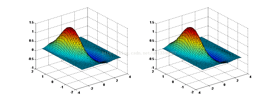
2、SVM中超平面的绘制

---

---

---

参考资料：
MatLab：meshgrid
Numpy中Meshgrid函数介绍及2种应用场景