移动机器人路径规划：人工势场法

article/2025/8/23 17:16:46

人工势场法是一种原理比较简单的移动机器人路径规划算法，它将目标点位置视做势能最低点，将地图中的障碍物视为势能高点，计算整个已知地图的势场图，然后理想情况下，机器人就像一个滚落的小球，自动避开各个障碍物滚向目标点。

参考：
源代码potential_field_planning.py
课件CMU RI 16-735机器人路径规划第4讲：人工势场法

具体地，目标点的势能公式为：

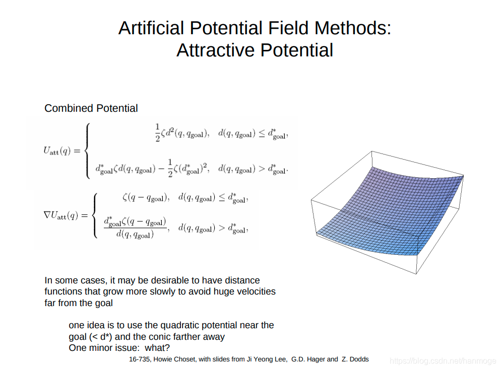
其中写道，为防止距离目标点较远时的速度过快，可以采用分段函数的形式描述，后文会进行展示。
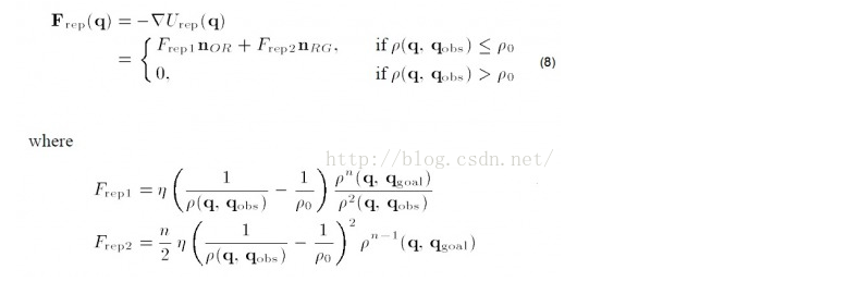
而障碍物的势能表示为：

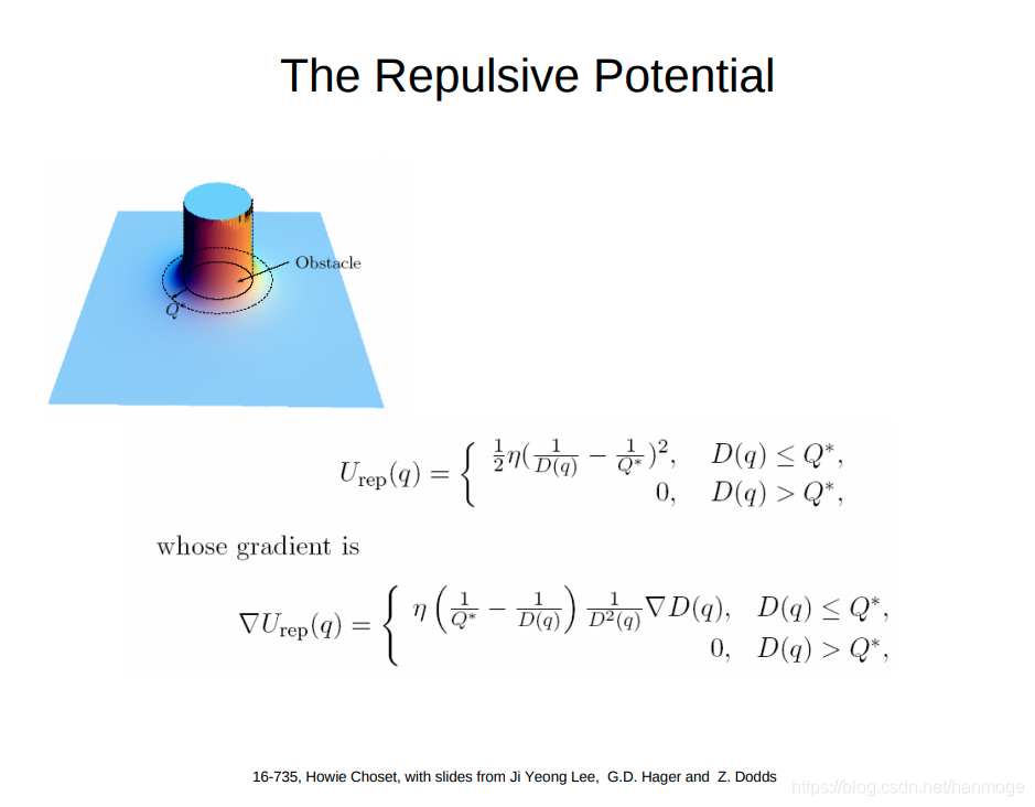
即在障碍物周围某个范围内具有高势能，范围外视障碍物的影响为0。
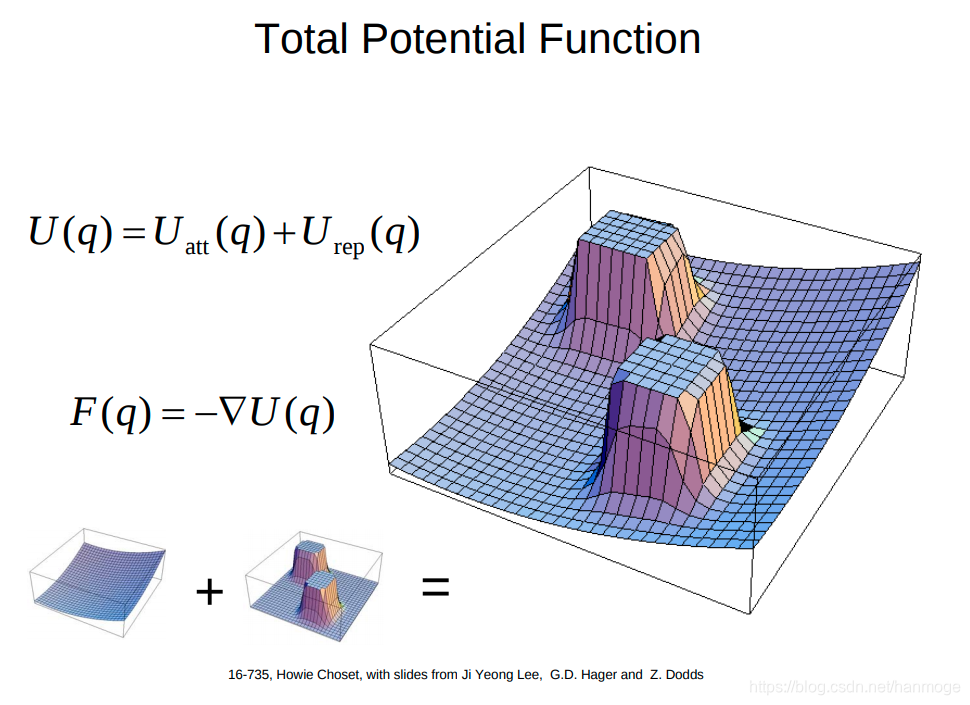
最终将目标点和障碍物的势能相加，获得整张势能地图：

以下是参考链接中的源代码，比较容易懂：

"""Potential Field based path plannerauthor: Atsushi Sakai (@Atsushi_twi)Ref:
https://www.cs.cmu.edu/~motionplanning/lecture/Chap4-Potential-Field_howie.pdf"""from collections import deque
import numpy as np
import matplotlib.pyplot as plt# Parameters
KP = 5.0  # attractive potential gain
ETA = 100.0  # repulsive potential gain
AREA_WIDTH = 30.0  # potential area width [m]
# the number of previous positions used to check oscillations
OSCILLATIONS_DETECTION_LENGTH = 3show_animation = Truedef calc_potential_field(gx, gy, ox, oy, reso, rr, sx, sy):"""计算势场图gx,gy: 目标坐标ox,oy: 障碍物坐标列表reso: 势场图分辨率rr: 机器人半径sx,sy: 起点坐标"""# 确定势场图坐标范围：minx = min(min(ox), sx, gx) - AREA_WIDTH / 2.0miny = min(min(oy), sy, gy) - AREA_WIDTH / 2.0maxx = max(max(ox), sx, gx) + AREA_WIDTH / 2.0maxy = max(max(oy), sy, gy) + AREA_WIDTH / 2.0# 根据范围和分辨率确定格数：xw = int(round((maxx - minx) / reso))yw = int(round((maxy - miny) / reso))# calc each potentialpmap = [[0.0 for i in range(yw)] for i in range(xw)]for ix in range(xw):x = ix * reso + minx   # 根据索引和分辨率确定x坐标for iy in range(yw):y = iy * reso + miny  # 根据索引和分辨率确定x坐标ug = calc_attractive_potential(x, y, gx, gy)  # 计算引力uo = calc_repulsive_potential(x, y, ox, oy, rr)  # 计算斥力uf = ug + uopmap[ix][iy] = ufreturn pmap, minx, minydef calc_attractive_potential(x, y, gx, gy):"""计算引力势能：1/2*KP*d"""return 0.5 * KP * np.hypot(x - gx, y - gy)def calc_repulsive_potential(x, y, ox, oy, rr):"""计算斥力势能：如果与最近障碍物的距离dq在机器人膨胀半径rr之内：1/2*ETA*(1/dq-1/rr)**2否则：0.0"""# search nearest obstacleminid = -1dmin = float("inf")for i, _ in enumerate(ox):d = np.hypot(x - ox[i], y - oy[i])if dmin >= d:dmin = dminid = i# calc repulsive potentialdq = np.hypot(x - ox[minid], y - oy[minid])if dq <= rr:if dq <= 0.1:dq = 0.1return 0.5 * ETA * (1.0 / dq - 1.0 / rr) ** 2else:return 0.0def get_motion_model():# dx, dy# 九宫格中 8个可能的运动方向motion = [[1, 0],[0, 1],[-1, 0],[0, -1],[-1, -1],[-1, 1],[1, -1],[1, 1]]return motiondef oscillations_detection(previous_ids, ix, iy):"""振荡检测：避免“反复横跳”"""previous_ids.append((ix, iy))if (len(previous_ids) > OSCILLATIONS_DETECTION_LENGTH):previous_ids.popleft()# check if contains any duplicates by copying into a setprevious_ids_set = set()for index in previous_ids:if index in previous_ids_set:return Trueelse:previous_ids_set.add(index)return Falsedef potential_field_planning(sx, sy, gx, gy, ox, oy, reso, rr):# calc potential fieldpmap, minx, miny = calc_potential_field(gx, gy, ox, oy, reso, rr, sx, sy)# search pathd = np.hypot(sx - gx, sy - gy)ix = round((sx - minx) / reso)iy = round((sy - miny) / reso)gix = round((gx - minx) / reso)giy = round((gy - miny) / reso)if show_animation:draw_heatmap(pmap)# for stopping simulation with the esc key.plt.gcf().canvas.mpl_connect('key_release_event',lambda event: [exit(0) if event.key == 'escape' else None])plt.plot(ix, iy, "*k")plt.plot(gix, giy, "*m")rx, ry = [sx], [sy]motion = get_motion_model()previous_ids = deque()while d >= reso:minp = float("inf")minix, miniy = -1, -1# 寻找8个运动方向中势场最小的方向for i, _ in enumerate(motion):inx = int(ix + motion[i][0])iny = int(iy + motion[i][1])if inx >= len(pmap) or iny >= len(pmap[0]) or inx < 0 or iny < 0:p = float("inf")  # outside areaprint("outside potential!")else:p = pmap[inx][iny]if minp > p:minp = pminix = inxminiy = inyix = minixiy = miniyxp = ix * reso + minxyp = iy * reso + minyd = np.hypot(gx - xp, gy - yp)rx.append(xp)ry.append(yp)# 振荡检测，以避免陷入局部最小值：if (oscillations_detection(previous_ids, ix, iy)):print("Oscillation detected at ({},{})!".format(ix, iy))breakif show_animation:plt.plot(ix, iy, ".r")plt.pause(0.01)print("Goal!!")return rx, rydef draw_heatmap(data):data = np.array(data).Tplt.pcolor(data, vmax=100.0, cmap=plt.cm.Blues)def main():print("potential_field_planning start")sx = 0.0  # start x position [m]sy = 10.0  # start y positon [m]gx = 30.0  # goal x position [m]gy = 30.0  # goal y position [m]grid_size = 0.5  # potential grid size [m]robot_radius = 5.0  # robot radius [m]# 以下障碍物坐标是我进行修改后的，用来展示人工势场法的困于局部最优的情况：ox = [15.0, 5.0, 20.0, 25.0, 12.0, 15.0, 19.0, 28.0, 27.0, 23.0, 30.0, 32.0]  # obstacle x position list [m]oy = [25.0, 15.0, 26.0, 25.0, 12.0, 20.0, 29.0, 28.0, 26.0, 25.0, 28.0, 27.0]  # obstacle y position list [m]if show_animation:plt.grid(True)plt.axis("equal")# path generation_, _ = potential_field_planning(sx, sy, gx, gy, ox, oy, grid_size, robot_radius)if show_animation:plt.show()if __name__ == '__main__':print(__file__ + " start!!")main()print(__file__ + " Done!!")

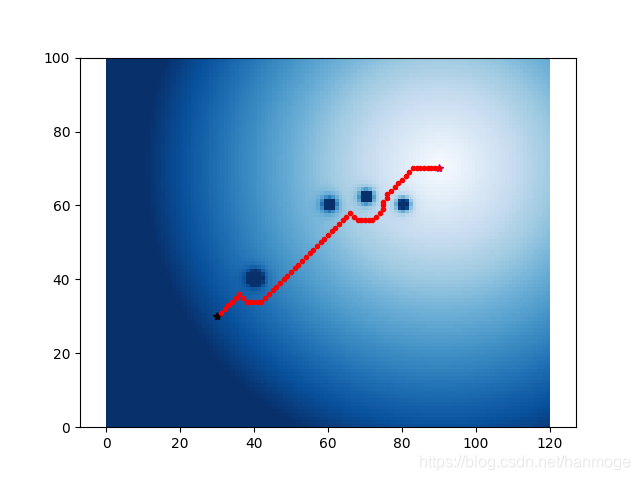
人工势场法的一项主要缺点就是可能会落入局部最优解，下图是源代码运行后的结果：

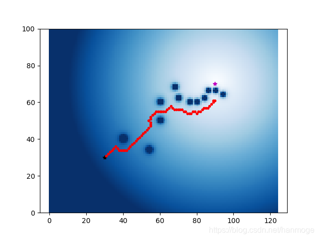
下面是在我添加了一些障碍物后，人工势场法困于局部最优解的情况：虽然还没有到达目标点，但势场决定了路径无法再前进。

需要注意的是，源代码在计算目标点势场的时候，使用的是某x，y位置距离目标点的距离的一次项，并未如课件中所示使用二次项，也是为了使势场变化没有那么快。下面是按照课件中所说，使用距离的二次项运行的结果，我们可以看到，为运行正常，KP需要调得很低：

KP = 0.1
def calc_attractive_potential(x, y, gx, gy):"""计算引力势能：1/2*KP*d^2"""return 0.5 * KP * np.hypot(x - gx, y - gy)**2

正常运行：

困在局部最优点：

可以从势场图中看到，引力变化较上一个例子快得多。

最后，我们将程序修改成上面课件截图中所示的分段函数：

KP = 0.25
dgoal = 10
def calc_attractive_potential(x, y, gx, gy):"""计算引力：如课件截图"""dg = np.hypot(x - gx, y - gy)if dg<=dgoal:U = 0.5 * KP * np.hypot(x - gx, y - gy)**2else:U = dgoal*KP*np.hypot(x - gx, y - gy) - 0.5*KP*dgoalreturn U